14  S: Linear Regression: Non-linear Transformations and Interactions

library(rethinking) # Load rethinking library to get data(Howell1)
library(rstanarm)   

Topics

• Non-linear relationships
  • logarithmic, exponential and power functions become linear after suitable log-transformations.
• Interaction
  • Between categorical variables (ANOVA type of data)
  • Between categorical and continuous variables
  • Between continuous variables
    • Linear interaction: Slope of one variable linearly related to another variable.

Readings:

Gelman et al. (2021), Chapter 10 (p. 134-) and 12 (p. 186-) illustrate interaction analysis using the kid_iq data. Chapter 16 (p. 301-) discusses sample size requirements (“power”) for interaction analysis.

14.1 Non-linear transformations

Non-linear transformations of predictor or outcome variables, e.g.,

• dichtomization, if coded 0 and 1, the regression coefficient has a simple interpretation, namely the difference in outcome between units coded 1 and units coded 0 (called treatment coding or dummy coding). Dichotomization may be a way to make variables of unknown scale level usable in regression analysis, e.g., a questionnaire item, with response alternative “not at all”, “little”, “moderately”, “much”, “very much”, maybe be coded 1 for those who answered “much” or “very much” and zero for the others.
• categorization, several categories, don’t forget to make them a factor if used as predictor in regression analysis.
• quadratic (as discussed last time), used to model curvilinear relationships, e.g., \(Happiness = b_0 + b_1age + b_2(age^2)\), people least happy in middle age (typically, Age would be centered in these analyses)
• log-transform, may normalize variables (or residuals) with positive skew
• log-transform and/or exponentiation of x and/or y-variables, to model logarithmic, exponential or or power law relationships between variables, as illustrated below (I used log base 2 in these illustrations just to make it easy to read: 1 unit increase is a doubling; Gelman et al. (2021) prefer the natural log, and I use this in the example in the weight and height example).

par(mfrow = c(3, 2))

# From logarithmic to linear
x <- 1:100
y <- log2(x)
plot(x, y, cex = 0.8, main = "Logarithmic function, y = log(x)")
lines(x, y, col = 'blue')
plot(log2(x), y, cex = 0.8)
lines(log2(x), y, col = 'blue')

# From exponential to linear
x <- seq(0.1, 4, by = 0.05)
y <- exp(x)
plot(x, y, cex = 0.8, main = "Exponential function, y = exp(x)")
lines(x, y, col = 'blue')
plot(x, log2(y), cex = 0.8)
lines(x, log2(y), col = 'blue')
# Or:
# plot(exp(x), y, cex = 0.8)
#lines(exp(x), y, col = 'blue')


# From power-law to linear
x <- seq(0.1, 10, by = 0.1)
y <- 1*x^(log2(1.5))  # Doubling of x increases y with 1.5
plot(x, y,  cex = 0.8, main = "Power function, y = x^b")
lines(x, y, col = 'blue')
plot(log2(x), log2(y),  cex = 0.8)
lines(log2(x), log2(y), col = 'blue')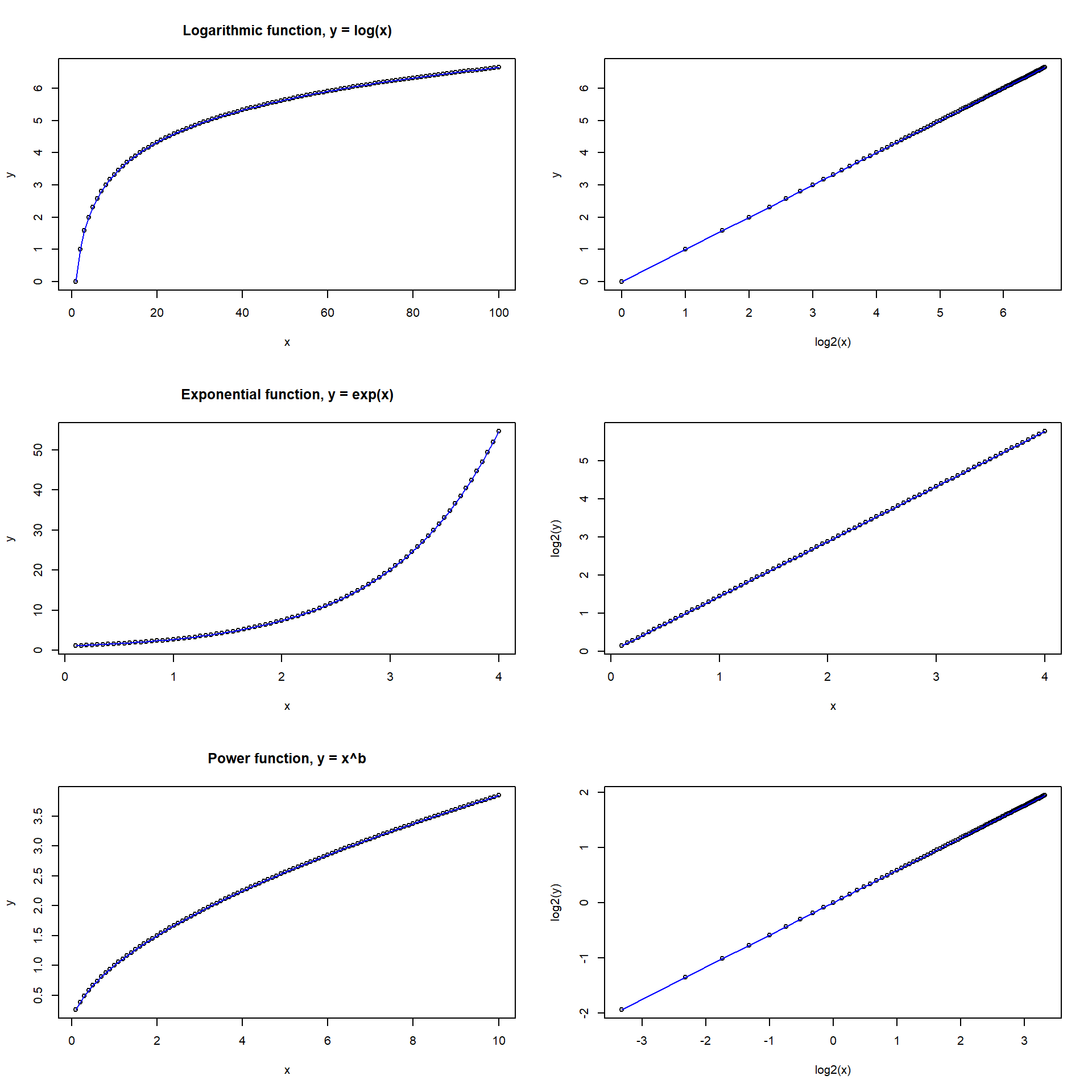

Non-linear trend turned linear, example

Here an example of a non-linear relationship that looks linear after log-transform. Anthropological data from the rethinking-package on height as a function of weight among children from a tribe in East Africa.

data(Howell1)  # From rethinking package
d <- Howell1
rm(Howell1)

# Only include children: < 18 years old
d2 <- d[d$age < 18, ]
summary(d2)

     height           weight            age              male       
 Min.   : 53.98   Min.   : 4.252   Min.   : 0.000   Min.   :0.0000  
 1st Qu.: 89.13   1st Qu.:11.708   1st Qu.: 3.000   1st Qu.:0.0000  
 Median :111.12   Median :16.981   Median : 7.000   Median :0.0000  
 Mean   :108.32   Mean   :18.414   Mean   : 7.722   Mean   :0.4792  
 3rd Qu.:127.72   3rd Qu.:23.417   3rd Qu.:12.000   3rd Qu.:1.0000  
 Max.   :158.12   Max.   :44.736   Max.   :17.000   Max.   :1.0000  

Linear fit doesn’t look too god!

par(mfrow = c(1, 2))
# Plot data and model predictions
plot(d2$weight, d2$height, xlab = "Weight [kg]", ylab = "Height [cm]")
mlin <- lm(height ~ weight, data = d2)
abline(mlin, col = "blue", lwd = 1.5)

# Residual plot
plot(mlin$fitted.values, mlin$residuals, 
     xlab = "Fitted values [cm]", ylab = "Residuals [cm]")
abline(0, 0, col = "black", lty = 2)
lines(lowess(mlin$fitted.values, mlin$residuals), col = "red", lty = 3)
mtext(side = 3, text = "Residual plot", cex = 0.9)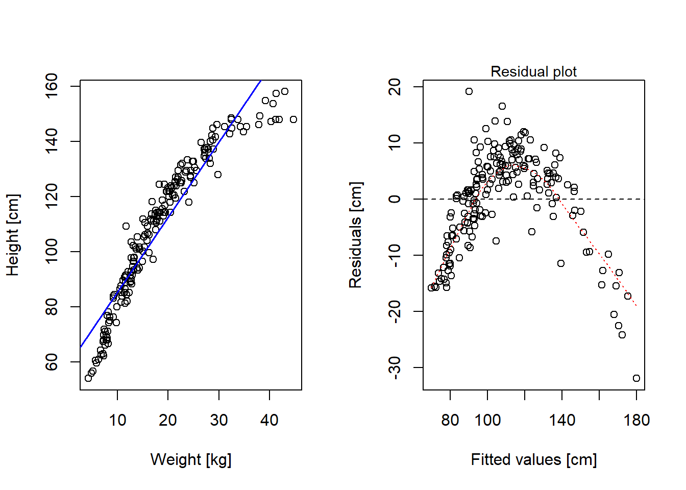

summary(mlin)

Call:
lm(formula = height ~ weight, data = d2)

Residuals:
    Min      1Q  Median      3Q     Max 
-31.960  -5.083   1.640   6.048  19.142 

Coefficients:
            Estimate Std. Error t value Pr(>|t|)    
(Intercept) 58.23060    1.40454   41.46   <2e-16 ***
weight       2.72009    0.06865   39.62   <2e-16 ***
---
Signif. codes:  0 '***' 0.001 '**' 0.01 '*' 0.05 '.' 0.1 ' ' 1

Residual standard error: 8.481 on 190 degrees of freedom
Multiple R-squared:  0.892, Adjusted R-squared:  0.8915 
F-statistic:  1570 on 1 and 190 DF,  p-value: < 2.2e-16

Looks better (but not perfect!) with log-weight as predictor

par(mfrow = c(1, 2))
# Plot in log units
plot(log(d2$weight), d2$height, xlab = "log(Weight [kg])", ylab = "Height [cm]")
mlog <- lm(height ~ log(weight), data = d2)
abline(mlog, col = "blue", lwd = 1.5)
summary(mlog)

Call:
lm(formula = height ~ log(weight), data = d2)

Residuals:
     Min       1Q   Median       3Q      Max 
-13.3503  -3.0401   0.2292   2.9634  17.7553 

Coefficients:
            Estimate Std. Error t value Pr(>|t|)    
(Intercept) -32.8566     1.9179  -17.13   <2e-16 ***
log(weight)  50.5309     0.6757   74.78   <2e-16 ***
---
Signif. codes:  0 '***' 0.001 '**' 0.01 '*' 0.05 '.' 0.1 ' ' 1

Residual standard error: 4.679 on 190 degrees of freedom
Multiple R-squared:  0.9671,    Adjusted R-squared:  0.967 
F-statistic:  5592 on 1 and 190 DF,  p-value: < 2.2e-16

# Plot in linear units
plot(d2$weight, d2$height, xlab = "Weight [kg]", ylab = "Height [cm]")
xline <- seq(1, 50, 0.1)
cflog <- mlog$coefficients
yline <- cflog[1] + cflog[2]*log(xline)
lines(xline, yline, col = "blue", lwd = 1.5)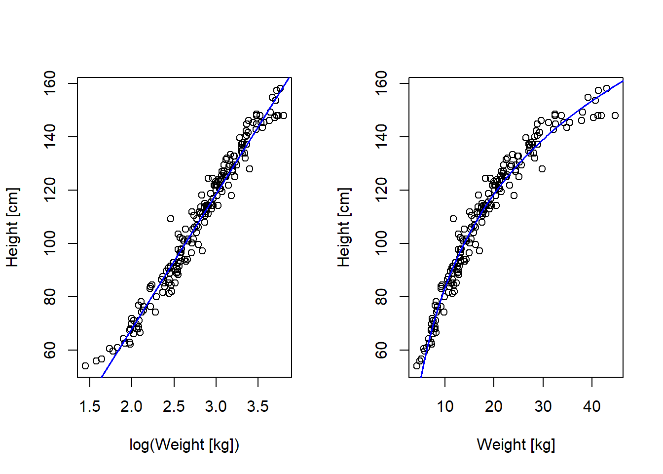

# Residual plot
plot(mlog$fitted.values, mlog$residuals, 
     xlab = "Fitted values [cm]", ylab = "Residuals [cm]")
abline(0, 0, col = "black", lty = 2)
lines(lowess(mlog$fitted.values, mlog$residuals), col = "red", lty = 3)
mtext(side = 3, text = "Residual plot", cex = 0.9)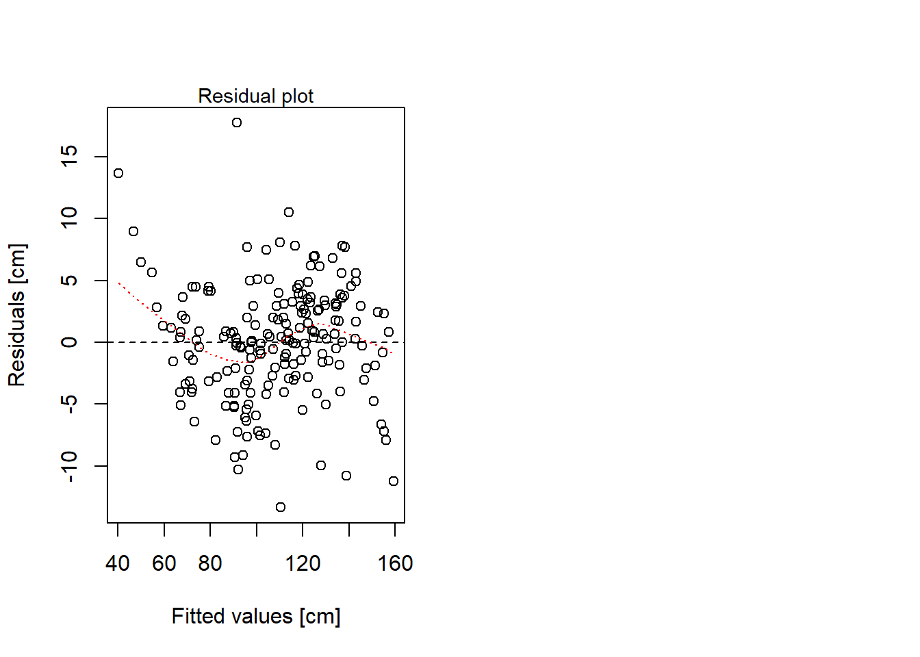

14.2 Interactions

We will again use the data set in kidiq.txt to illustrate several points below. The data is from a survey of adult American women and their children. Gelman et al. (2021) describe the data set and use it at several places, e.g pp. 130-136, 156-158, 161, 185-187, and 197.

Code book:

• kid_score  Test score children, on IQ-like measure (in the sample with mean and standard deviation of 87 and 20 points, respectively).
• mom_hs  Indicator variable: mother did complete high-school (1) or not (0)
• mom_iq  Test score mothers, transformed to IQ score: mean = 100, sd = 15.
• mom_work  Working status of mother, coded 1-4:
  • 1: mother did not work in first three years of child’s life,
  • 2: mother worked in second or third year of child’s life,
  • 3: mother worked part-time in first year of child’s life,
  • 4: mother worked full-time in first year of child’s life.
• mom_age Age of mothers, years

Import data and transform variables:

d <- read.table("./datasets/kidiq.txt", sep = ",", header = TRUE)

# Dichotomize mothers IQ (above mean = 1, below mean = 0), to be used as 
# indicator variable in regression analysis
d$mom_iq_hi <- 1 * (d$mom_iq > mean(d$mom_iq))

# Center mom_iq to be used as continuous variable in regression analysis
d$mom_iq_c <- d$mom_iq - mean(d$mom_iq)

# Center mom_age to mean age 
d$mom_age_c <- d$mom_age - mean(d$mom_age)

# Factor variable of mom_work
d$mom_work_f <- factor(d$mom_work, levels = c(1, 2, 3, 4),
                       labels = c("1_nowork", "2_worky2y3", 
                                  "3_parttime", "4_fulltime"))

# Linear transform kid_score to iq-scale: mean = 100, sd = 15
# Can be done in one step, I prefer to do it in two steps, via z-scores
zkid <- (d$kid_score - mean(d$kid_score)) / sd(d$kid_score)
d$kid_iq <- zkid * 15 + 100

str(d)

'data.frame':   434 obs. of  10 variables:
 $ kid_score : int  65 98 85 83 115 98 69 106 102 95 ...
 $ mom_hs    : int  1 1 1 1 1 0 1 1 1 1 ...
 $ mom_iq    : num  121.1 89.4 115.4 99.4 92.7 ...
 $ mom_work  : int  4 4 4 3 4 1 4 3 1 1 ...
 $ mom_age   : int  27 25 27 25 27 18 20 23 24 19 ...
 $ mom_iq_hi : num  1 0 1 0 0 1 1 1 0 0 ...
 $ mom_iq_c  : num  21.12 -10.64 15.44 -0.55 -7.25 ...
 $ mom_age_c : num  4.21 2.21 4.21 2.21 4.21 ...
 $ mom_work_f: Factor w/ 4 levels "1_nowork","2_worky2y3",..: 4 4 4 3 4 1 4 3 1 1 ...
 $ kid_iq    : num  84 108.2 98.7 97.2 120.7 ...

Interaction analysis with two categorical variables

Factorial designs include all combinations of the levels of two (or more) categorical variables. They are often used for interaction analyses.

Here illustrated with two dichotomous variables as predictors, mom_hs and mom_iq_hi, essentially a 2x2 between-participant ANOVA with kid_iq as outcome. Below sample sizes and statistics for kid_iq split by predictors:

my_stat <- function(x) {
  n <- length(x)
  m <- mean(x, na.rm = TRUE)
  s <- sd(x, na.rm = TRUE)
  se <- s/sqrt(length(x))
  out <- c(n = n, m = m, sd = s, se = se)
  out
}

ss <- aggregate(list(kid_iq = d$kid_iq), 
          list(mom_hs = d$mom_hs, mom_iqhi = d$mom_iq_hi), 
          my_stat)
round(ss, 1)

  mom_hs mom_iqhi kid_iq.n kid_iq.m kid_iq.sd kid_iq.se
1      0        0     71.0     88.7      15.3       1.8
2      1        0    168.0     97.4      13.9       1.1
3      0        1     22.0    107.6      11.8       2.5
4      1        1    173.0    106.2      12.7       1.0

Fit regression model:

\(y_i = Normal(\mu_i, \sigma)\)

\(\mu_i = b_0 + b_1D_i + b_2G_i + b_3D_iG_i\),

where D is the dichotomous mom_hs variable and G is the dichotomous mom_iq_hi variable.

This linear model can be broken down in four parts, one for each of the 2x2 combinations of predictors:

mom_hs	mom_iq_hi	predicted mean	observed mean
0	0	\(b_0\)	88.7
1	0	\(b_0 + b_1\)	97.4
0	1	\(b_0 + b_2\)	107.6
1	1	\(b_0 + b_1 + b_2 + b_3\)	106.2

Fit model

d_interact <- glm(kid_iq ~ mom_hs + mom_iq_hi + mom_hs*mom_iq_hi, data = d)
summary(d_interact)

Call:
glm(formula = kid_iq ~ mom_hs + mom_iq_hi + mom_hs * mom_iq_hi, 
    data = d)

Coefficients:
                 Estimate Std. Error t value Pr(>|t|)    
(Intercept)        88.742      1.612  55.056  < 2e-16 ***
mom_hs              8.624      1.923   4.486 9.32e-06 ***
mom_iq_hi          18.856      3.314   5.690 2.36e-08 ***
mom_hs:mom_iq_hi  -10.012      3.626  -2.761  0.00601 ** 
---
Signif. codes:  0 '***' 0.001 '**' 0.01 '*' 0.05 '.' 0.1 ' ' 1

(Dispersion parameter for gaussian family taken to be 184.4612)

    Null deviance: 97425  on 433  degrees of freedom
Residual deviance: 79318  on 430  degrees of freedom
AIC: 3502

Number of Fisher Scoring iterations: 2

confint(d_interact)

Waiting for profiling to be done...

                      2.5 %   97.5 %
(Intercept)       85.583239 91.90156
mom_hs             4.856419 12.39250
mom_iq_hi         12.360588 25.35126
mom_hs:mom_iq_hi -17.118388 -2.90527

Visualize model

# Empty plot
plot(d$mom_iq_hi, d$kid_iq, pch = '', xlim = c(-0.2, 1.2), ylim = c(50, 150),
     axes = FALSE, xlab = "Mother IQ below (0) or above (1) average",
     ylab = "Kid IQ")

# Add data points, with some jitter along x for visibility
offset <- 0.02
j0 <- rnorm(length(d$mom_iq_hi[d$mom_hs == 0]), -offset, 0.01)  # x-jitter
j1 <- rnorm(length(d$mom_iq_hi[d$mom_hs == 1]), offset, 0.01)  # x-jitter
points(d$mom_iq_hi[d$mom_hs == 0] + j0, d$kid_iq[d$mom_hs == 0], 
       pch = 21, bg = "blue")
points(d$mom_iq_hi[d$mom_hs == 1] + j1, d$kid_iq[d$mom_hs == 1],
       pch = 21, bg = "white")

# Add axis
axis(1, at = c(-0.2, 0, 1, 1.2), labels = c("", "0", "1", ""), pos = 50)
axis(2, at = seq(50, 150, 10), pos = -0.2, las = 2)

# Add regression lines
cf <- d_interact$coefficients
xline <- c(0, 1)
yline0 <- c(cf[1], cf[1] + cf[3])
yline1 <- c(cf[1] + cf[2], sum(cf))
lines(xline - offset, yline0, col = "blue")
lines(xline + offset, yline1, lty = 2)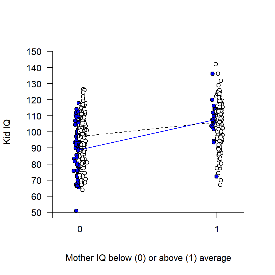

Compare with Analysis of variance (ANOVA), same analysis but less informative output. (aov() would be exactly the same as using lm() and another set of contrasts)

a1 <- aov(kid_iq ~ mom_hs + mom_iq_hi + mom_hs:mom_iq_hi, data = d)
summary(a1)

                  Df Sum Sq Mean Sq F value   Pr(>F)    
mom_hs             1   5468    5468  29.645 8.74e-08 ***
mom_iq_hi          1  11232   11232  60.890 4.63e-14 ***
mom_hs:mom_iq_hi   1   1406    1406   7.624  0.00601 ** 
Residuals        430  79318     184                     
---
Signif. codes:  0 '***' 0.001 '**' 0.01 '*' 0.05 '.' 0.1 ' ' 1

Coefficients and confidence intervals from ANOVA model

a1$coefficients

     (Intercept)           mom_hs        mom_iq_hi mom_hs:mom_iq_hi 
       88.742397         8.624461        18.855922       -10.011829 

confint(a1)

                      2.5 %    97.5 %
(Intercept)       85.574322 91.910472
mom_hs             4.845784 12.403138
mom_iq_hi         12.342254 25.369591
mom_hs:mom_iq_hi -17.138447 -2.885211

Interaction analysis with one categorical and one continuous variable

Let’s start with an additive model, using mom_hs and mom_iq as independent variables

\(y_i = Normal(\mu_i, \sigma)\)

\(\mu_i = b_0 + b_1D_i + b_2x_i\),

where D is the dichotomous mom_hs variable and x is the continuous variable mom_iq.

Fit model, using glm():

# Adjusted: + mom_iq
m1 <- glm(kid_iq ~ mom_hs + mom_iq_c, data = d)
summary(m1)

Call:
glm(formula = kid_iq ~ mom_hs + mom_iq_c, data = d)

Coefficients:
            Estimate Std. Error t value Pr(>|t|)    
(Intercept) 96.56423    1.42844  67.601  < 2e-16 ***
mom_hs       4.37279    1.62548   2.690  0.00742 ** 
mom_iq_c     0.41442    0.04452   9.309  < 2e-16 ***
---
Signif. codes:  0 '***' 0.001 '**' 0.01 '*' 0.05 '.' 0.1 ' ' 1

(Dispersion parameter for gaussian family taken to be 177.6375)

    Null deviance: 97425  on 433  degrees of freedom
Residual deviance: 76562  on 431  degrees of freedom
AIC: 3484.6

Number of Fisher Scoring iterations: 2

Visualize additive model:

## Draw figure of additive model

# Empty plot
plot(d$mom_iq_c, d$kid_iq, axes = FALSE, pch = "",
     xlim = c(-30, 40), ylim = c(50, 150), xlab = "Mother IQ", ylab = "Kid IQ")
# Add points for mom_hs = 0 (blue) and mom_hs = 1 )(white)
points(d$mom_iq_c[d$mom_hs == 0], d$kid_iq[d$mom_hs == 0], 
       pch = 21, bg = "blue")
points(d$mom_iq_c[d$mom_hs == 1], d$kid_iq[d$mom_hs == 1], 
       pch = 21, bg = "white")
# Add regression lines
cf <- m1$coefficients  # Coefficients of model
xline <- c(-30, 40)  # Two points along the x-axis
yline0 <- cf[1] + cf[3]*xline # Predictions for mom_hs = 0
yline1 <- cf[1] + cf[2] + cf[3]*xline # Predictions for mom_hs = 1
lines(xline, yline0 , col = "blue")
lines(xline, yline1 , col = "black", lty = 3)

# Confidence bands around regression line (+- 2SE of predicted mean) --
# Calculate CI-bands mom_hs = 0  
xline <- seq(-30, 40, 0.1)
hs0 <- rep(0, length(xline))
newdata0 <- data.frame(mom_iq_c = xline, mom_hs = hs0)
predict0 <- predict(m1, newdata=newdata0, se.fit = TRUE)
ci0lo <- predict0$fit - 2*predict0$se.fit
ci0hi <- predict0$fit + 2*predict0$se.fit

# Shade area mom_hs = 0 
polygon(x = c(xline, rev(xline)), y = c(ci0lo, rev(ci0hi)), 
        col =  rgb(0, 0, 1, 0.1), border = FALSE)      

# Calculate CI-bands mom_hs = 1 
hs1 <- rep(1, length(xline))
newdata1 <- data.frame(mom_iq_c = xline, mom_hs = hs1)
predict1 <- predict(m1, newdata=newdata1, se.fit = TRUE)
ci1lo <- predict1$fit - 1.96*predict1$se.fit
ci1hi <- predict1$fit + 1.96*predict1$se.fit


# Shade area mom_hs = 1 
polygon(x = c(xline, rev(xline)), y = c(ci1lo, rev(ci1hi)), 
        col =  rgb(0, 0, 0, 0.1), border = FALSE)  # shaded area
# ---

# Add axis (transforming back mom_iq to mean = 100)
axis(1, at = seq(-30, 40, 10), 
     labels = seq(-30, 40, 10) + mean(d$mom_iq), # Transforming back to mom_iq
     pos = 50) 
axis(2, at = seq(50, 150, 10), las = 2, pos = -30)

# Add legend
points(-25, 148, pch = 21, bg = "blue", cex = 0.8)
points(-25, 143, pch = 21, bg = "white", cex = 0.8)
text(x = -25, y = 148, labels = "Mother did not complete high-school", 
     pos = 4, cex = 0.7)
text(x = -25, y = 143, labels = "Mother completed high-school", 
     pos = 4, cex = 0.7)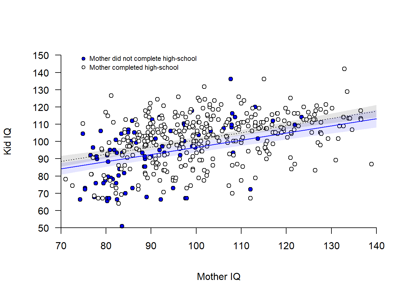

The model implies parallel lines, but the data seem to suggest that a steeper slope should be considered for mom_hs = 0 (blue points) compared to for mom_hs = 1 (white points). Different slope is the same as an interaction, so let’s add an interaction term:

\(y_i = Normal(\mu_i, \sigma)\)

\(\mu_i = b_0 + b_1D_i + b_2x_i + b_3D_ix_i\).

Fit model with interaction:

m1_interact <- glm(kid_iq ~ mom_hs + mom_iq_c + mom_hs:mom_iq_c, data = d)
summary(m1_interact)

Call:
glm(formula = kid_iq ~ mom_hs + mom_iq_c + mom_hs:mom_iq_c, data = d)

Coefficients:
                Estimate Std. Error t value Pr(>|t|)    
(Intercept)      98.9782     1.6302  60.716  < 2e-16 ***
mom_hs            2.0877     1.7834   1.171  0.24239    
mom_iq_c          0.7120     0.1090   6.531 1.84e-10 ***
mom_hs:mom_iq_c  -0.3559     0.1192  -2.985  0.00299 ** 
---
Signif. codes:  0 '***' 0.001 '**' 0.01 '*' 0.05 '.' 0.1 ' ' 1

(Dispersion parameter for gaussian family taken to be 174.4352)

    Null deviance: 97425  on 433  degrees of freedom
Residual deviance: 75007  on 430  degrees of freedom
AIC: 3477.7

Number of Fisher Scoring iterations: 2

confint(m1_interact)

Waiting for profiling to be done...

                     2.5 %      97.5 %
(Intercept)     95.7831137 102.1733465
mom_hs          -1.4076660   5.5830621
mom_iq_c         0.4983719   0.9257190
mom_hs:mom_iq_c -0.5895545  -0.1222411

Visualize interaction model:

m1_interact <- glm(kid_iq ~ mom_hs + mom_iq_c + mom_hs:mom_iq_c, data = d)
summary(m1_interact)

Call:
glm(formula = kid_iq ~ mom_hs + mom_iq_c + mom_hs:mom_iq_c, data = d)

Coefficients:
                Estimate Std. Error t value Pr(>|t|)    
(Intercept)      98.9782     1.6302  60.716  < 2e-16 ***
mom_hs            2.0877     1.7834   1.171  0.24239    
mom_iq_c          0.7120     0.1090   6.531 1.84e-10 ***
mom_hs:mom_iq_c  -0.3559     0.1192  -2.985  0.00299 ** 
---
Signif. codes:  0 '***' 0.001 '**' 0.01 '*' 0.05 '.' 0.1 ' ' 1

(Dispersion parameter for gaussian family taken to be 174.4352)

    Null deviance: 97425  on 433  degrees of freedom
Residual deviance: 75007  on 430  degrees of freedom
AIC: 3477.7

Number of Fisher Scoring iterations: 2

confint(m1_interact)

Waiting for profiling to be done...

                     2.5 %      97.5 %
(Intercept)     95.7831137 102.1733465
mom_hs          -1.4076660   5.5830621
mom_iq_c         0.4983719   0.9257190
mom_hs:mom_iq_c -0.5895545  -0.1222411

# Empty plot
plot(d$mom_iq_c, d$kid_iq, axes = FALSE, pch = "",
     xlim = c(-30, 40), ylim = c(50, 150), xlab = "Mother IQ", ylab = "Kid IQ")
# Add points for mom_hs = 0 (blue) and mom_hs = 1 )(white)
points(d$mom_iq_c[d$mom_hs == 0], d$kid_iq[d$mom_hs == 0], 
       pch = 21, bg = "blue")
points(d$mom_iq_c[d$mom_hs == 1], d$kid_iq[d$mom_hs == 1], 
       pch = 21, bg = "white")

# Add regression lines
cf <- m1_interact$coefficients  # Coefficients of model
xline <- c(-30, 40)  # Two points along the x-axis
yline0 <- cf[1] + cf[3]*xline # Predictions for mom_hs = 0
yline1 <- cf[1] + cf[2] + (cf[3]+cf[4])*xline # Predictions for mom_hs = 1
lines(xline, yline0 , col = "blue")
lines(xline, yline1 , col = "black", lty = 3)

# Add axis (transforming back mom_iq to mean = 100)
axis(1, at = seq(-30, 40, 10), 
     labels = seq(-30, 40, 10) + mean(d$mom_iq), # Transforming back to mom_iq
     pos = 50) 
axis(2, at = seq(50, 150, 10), las = 2, pos = -30)

# Add legend
points(-25, 148, pch = 21, bg = "blue", cex = 0.8)
points(-25, 143, pch = 21, bg = "white", cex = 0.8)
text(x = -25, y = 148, labels = "Mother did not complete high-school", 
     pos = 4, cex = 0.7)
text(x = -25, y = 143, labels = "Mother completed high-school", 
     pos = 4, cex = 0.7)

# Confidence bands around regression line (+/- 2SE of predicted mean)
# Calculate CI-bands mom_hs = 0  
xline <- seq(-30, 40, 0.1)
hs0 <- rep(0, length(xline))
newdata0 <- data.frame(mom_iq_c = xline, mom_hs = hs0)
predict0 <- predict(m1_interact, newdata=newdata0, se.fit = TRUE)
ci0lo <- predict0$fit - 2*predict0$se.fit
ci0hi <- predict0$fit + 2*predict0$se.fit

# Shade area mom_hs = 0 
polygon(x = c(xline, rev(xline)), y = c(ci0lo, rev(ci0hi)), 
        col =  rgb(0, 0, 1, 0.1), border = FALSE)      

# Calculate CI-bands mom_hs = 1 
hs1 <- rep(1, length(xline))
newdata1 <- data.frame(mom_iq_c = xline, mom_hs = hs1)
predict1 <- predict(m1_interact, newdata=newdata1, se.fit = TRUE)
ci1lo <- predict1$fit - 1.96*predict1$se.fit
ci1hi <- predict1$fit + 1.96*predict1$se.fit

# Shade area mom_hs = 1 
polygon(x = c(xline, rev(xline)), y = c(ci1lo, rev(ci1hi)), 
        col =  rgb(0, 0, 0, 0.1), border = FALSE)  # shaded area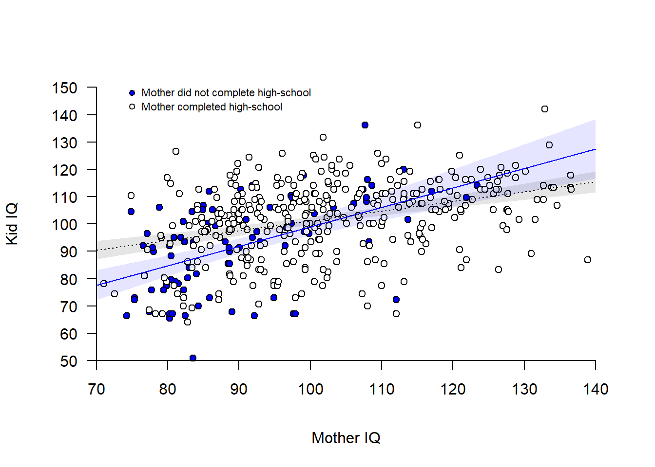

Please compare the interaction model to doing two separate regression analysis, one for each of the two groups defined by mom_hs. Note that this allows different \(\sigma\) for the two groups, otherwise coefficients should be very similar.

Bivariate model for kids to mothers who did not complete high-school:

\(y_i = Normal(\mu_i, \sigma)\)

\(\mu_i = a_0 + a_1x_i, \ \ \ \ D_i = 0\),

# Data frame with only mom_hs == 0
hs0 <- d[d$mom_hs == 0, ]  
m_hs0 <- glm(kid_iq ~ mom_iq_c, data = hs0)
m_hs0

Call:  glm(formula = kid_iq ~ mom_iq_c, data = hs0)

Coefficients:
(Intercept)     mom_iq_c  
     98.978        0.712  

Degrees of Freedom: 92 Total (i.e. Null);  91 Residual
Null Deviance:      25320 
Residual Deviance: 17880    AIC: 759

confint(m_hs0)

Waiting for profiling to be done...

                 2.5 %      97.5 %
(Intercept) 95.5873044 102.3691558
mom_iq_c     0.4852771   0.9388138

… and bivariate model for kids to mothers who did complete high-school

\(y_i = Normal(\mu_i, \sigma)\)

\(\mu_i = g_0 + g_1x_i, \ \ \ \ D_i = 1\).

# Data frame with only mom_hs == 1
hs1 <- d[d$mom_hs == 1, ]  
m_hs1 <- glm(kid_iq ~ mom_iq_c, data = hs1)
m_hs1

Call:  glm(formula = kid_iq ~ mom_iq_c, data = hs1)

Coefficients:
(Intercept)     mom_iq_c  
   101.0659       0.3561  

Degrees of Freedom: 340 Total (i.e. Null);  339 Residual
Null Deviance:      66640 
Residual Deviance: 57130    AIC: 2720

confint(m_hs1)

Waiting for profiling to be done...

                 2.5 %      97.5 %
(Intercept) 99.6728441 102.4590121
mom_iq_c     0.2632179   0.4490773

Interaction analysis with two continous variables

Linear interaction: Slope of one variable linearly related to another variable:

\(Y = a_0 + a_1X_1 + a_2X_2\), and
\(a_1 = b_0 + b_1X_2\)

Combining these two gives:
\(Y = a_0 + (b_0 + b_1X_2)X_1 + a_2X_2\)
\(Y = a_0 + (b_0X_1 + b_1X_2X_1) + a_2X_2\)
\(Y = a_0 + b_0X_1 + a_2X_2 + b_1X_1X_2\)

The same would have been obtained had slope of \(X_2\) been linearly related to slope of \(X_1\).

Here an example with mom_iq and mom_age as continuous variables in an interaction analysis. It is generally a good idea to use centered predictors.

m2 <- glm(kid_iq ~ mom_iq_c + mom_age_c + mom_iq_c:mom_age_c, data = d)
summary(m2)

Call:
glm(formula = kid_iq ~ mom_iq_c + mom_age_c + mom_iq_c:mom_age_c, 
    data = d)

Coefficients:
                    Estimate Std. Error t value Pr(>|t|)    
(Intercept)        100.05798    0.64674 154.711   <2e-16 ***
mom_iq_c             0.45122    0.04386  10.288   <2e-16 ***
mom_age_c            0.31029    0.24107   1.287    0.199    
mom_iq_c:mom_age_c  -0.01566    0.01584  -0.989    0.323    
---
Signif. codes:  0 '***' 0.001 '**' 0.01 '*' 0.05 '.' 0.1 ' ' 1

(Dispersion parameter for gaussian family taken to be 180.0384)

    Null deviance: 97425  on 433  degrees of freedom
Residual deviance: 77417  on 430  degrees of freedom
AIC: 3491.5

Number of Fisher Scoring iterations: 2

confint(m2)

Waiting for profiling to be done...

                         2.5 %       97.5 %
(Intercept)        98.79039224 101.32557605
mom_iq_c            0.36526144   0.53718097
mom_age_c          -0.16220394   0.78277753
mom_iq_c:mom_age_c -0.04670478   0.01538788

Visualize model, always needed to understand the meaning of linear interactions. Here illustrated in separate plots for low, medium and high levels of age.

# User-made plot functions
empty_plot <- function() {
  # Empty plot
plot(d$mom_iq_c, d$kid_iq, axes = FALSE, pch = "",
     xlim = c(-30, 40), ylim = c(80, 130), xlab = "Mother IQ", ylab = "Kid IQ")
}

add_data <- function(a) {
  
  # points(d$mom_iq_c, d$kid_iq, pch = 21, bg = "grey")

  # Add confidence band : +/- 2SE
  cf <- m2$coefficientscf 
  xline <- seq(-30, 40, 0.1)
  age <- rep(a, length(xline)) # age_c  = a 
  newdata <- data.frame(mom_iq_c = xline, mom_age_c = age)
  mm <- predict(m2, newdata = newdata)
  pred <- predict(m2, newdata = newdata, se.fit = TRUE)
  cilo <- pred$fit - 2*pred$se.fit
  cihi <- pred$fit + 2*pred$se.fit
  polygon(x = c(xline, rev(xline)), y = c(cilo, rev(cihi)), 
        col =  rgb(0, 0, 0, 0.1), border = FALSE)  # shaded area
  
  # Add regression line
  lines(xline, mm, lty = 2)
  
  # Add axis (transforming back mom_iq to mean = 100)
  axis(1, at = seq(-30, 40, 20), 
     labels = seq(-30, 40, 20) + mean(d$mom_iq), # Transforming back to mom_iq
     pos = 80) 
  axis(2, at = seq(50, 150, 10), las = 2, pos = -30)
}

# Draw three plots
par(mfrow = c(1, 3))

# age_c =  -2, approx 21 y
empty_plot()
add_data(a = -4)
text(-10, 125, "Mother's age 19 y", cex = 1, pos = 4)

# age_c =  0, approx 23 y
empty_plot()
add_data(a = 0)
text(-10, 125, "Mother's age 23 y", cex = 1, pos = 4)

# age_c =  2, approx 25 y
empty_plot()
add_data(a = 4)
text(-10, 125, "Mother's age 27 y", cex = 1, pos = 4)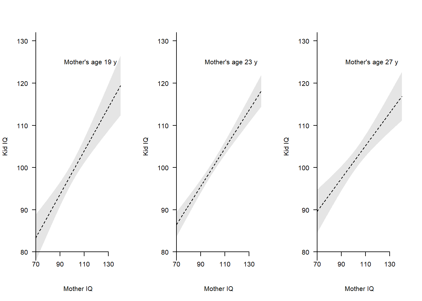

Figure clearly shows similar slopes for the three age groups, in line with the regression output suggesting no strong linear interaction.

Practice

The practice problems are labeled Easy (E), Medium (M), and Hard (H), (as in McElreath (2020)).

Easy

14E1. Give examples of when you would consider to log-transform …

1. A predictor variable.
2. An outcome variable.

14E2.
Below is a plot of age and waist circumference in a sample of Swedish women (open circles) and men (filled circles). The lines show the fit of the linear model

\(Waist = b_0 + b_1(Age-20) + b_2Male + b_3((Age-20)*Male)\),

where \(Waist\) is waist circumference in centimeters, \(Age\) is in years and \(Male\) is an indicator variable coded 0 for women and 1 for men. The solid line is for women (\(Male = 0\)) and the dashed line for men (\(Male = 1\))

Estimate by eye the four coefficients \(b_0, ..., b_3\)

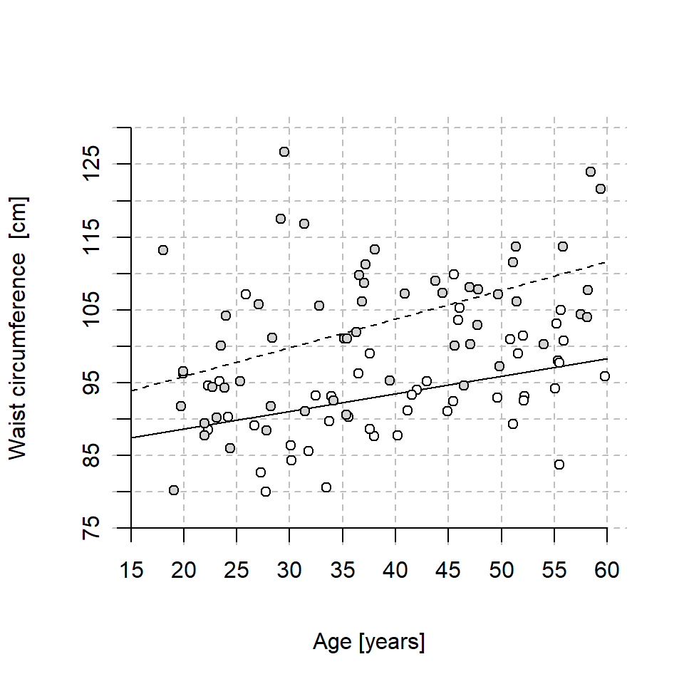
14E3.
The figure in 14E2 has two lines.

\(y = a_0 + a_1Age\) for females (solid line), and

\(y = d_0 + d_1Age\) for males (dotted line).

Relate each of these coefficients (\(a_0, a_1, d_0, d_1\)) to the coefficients of the fitted model \(b_0, b_1, b_2, b_3\) displayed in 14E2.

Here is the model fit from 14E2!

round(cf, 1)

(Intercept)       age20        male  age20:male 
       88.7         0.2         7.2         0.2 

Medium

14M1. Interactions should always be understood in relation to the statistical model. An interaction with the outcome in linear units may not be present if the outcome is modeled in log-units. Explain and visualize.

Hard

14H1. Use stan_glm() to fit the interaction model above: kid_iq ~ mom_hs + mom_iq_c + mom_hs:mom_iq_c and draw the figure with CI-bands around model predictions (x-axis: mom_iq (non-centered!), separate lines for mom_hs)

(Session Info)

sessionInfo()

R version 4.4.2 (2024-10-31 ucrt)
Platform: x86_64-w64-mingw32/x64
Running under: Windows 11 x64 (build 26100)

Matrix products: default


locale:
[1] LC_COLLATE=Swedish_Sweden.utf8  LC_CTYPE=Swedish_Sweden.utf8   
[3] LC_MONETARY=Swedish_Sweden.utf8 LC_NUMERIC=C                   
[5] LC_TIME=Swedish_Sweden.utf8    

time zone: Europe/Stockholm
tzcode source: internal

attached base packages:
[1] parallel  stats     graphics  grDevices utils     datasets  methods  
[8] base     

other attached packages:
[1] rstanarm_2.32.1     Rcpp_1.0.14         rethinking_2.42    
[4] posterior_1.6.1     cmdstanr_0.9.0.9000

loaded via a namespace (and not attached):
 [1] tidyselect_1.2.1     dplyr_1.1.4          farver_2.1.2        
 [4] loo_2.8.0            fastmap_1.2.0        tensorA_0.36.2.1    
 [7] shinystan_2.6.0      promises_1.3.3       shinyjs_2.1.0       
[10] digest_0.6.37        mime_0.13            lifecycle_1.0.4     
[13] StanHeaders_2.32.10  survival_3.7-0       processx_3.8.6      
[16] magrittr_2.0.3       compiler_4.4.2       rlang_1.1.6         
[19] tools_4.4.2          igraph_2.1.4         yaml_2.3.10         
[22] knitr_1.50           htmlwidgets_1.6.4    pkgbuild_1.4.8      
[25] curl_6.4.0           plyr_1.8.9           RColorBrewer_1.1-3  
[28] dygraphs_1.1.1.6     abind_1.4-8          miniUI_0.1.2        
[31] grid_4.4.2           stats4_4.4.2         xts_0.14.1          
[34] xtable_1.8-4         inline_0.3.21        ggplot2_3.5.2       
[37] scales_1.4.0         gtools_3.9.5         MASS_7.3-61         
[40] cli_3.6.5            mvtnorm_1.3-3        rmarkdown_2.29      
[43] reformulas_0.4.1     generics_0.1.4       RcppParallel_5.1.10 
[46] rstudioapi_0.17.1    reshape2_1.4.4       minqa_1.2.8         
[49] rstan_2.32.7         stringr_1.5.1        splines_4.4.2       
[52] shinythemes_1.2.0    bayesplot_1.13.0     matrixStats_1.5.0   
[55] base64enc_0.1-3      vctrs_0.6.5          boot_1.3-31         
[58] Matrix_1.7-1         V8_6.0.4             jsonlite_2.0.0      
[61] crosstalk_1.2.1      glue_1.8.0           nloptr_2.2.1        
[64] codetools_0.2-20     ps_1.9.1             DT_0.33             
[67] distributional_0.5.0 stringi_1.8.7        shape_1.4.6.1       
[70] gtable_0.3.6         later_1.4.2          QuickJSR_1.8.0      
[73] lme4_1.1-37          tibble_3.3.0         colourpicker_1.3.0  
[76] pillar_1.10.2        htmltools_0.5.8.1    R6_2.6.1            
[79] Rdpack_2.6.4         evaluate_1.0.3       shiny_1.11.1        
[82] lattice_0.22-6       markdown_2.0         rbibutils_2.3       
[85] backports_1.5.0      threejs_0.3.4        httpuv_1.6.16       
[88] rstantools_2.4.0     nlme_3.1-166         coda_0.19-4.1       
[91] gridExtra_2.3        checkmate_2.3.2      xfun_0.52           
[94] zoo_1.8-14           pkgconfig_2.0.3     

Gelman, A., Hill, J., & Vehtari, A. (2021). Regression and other stories. Cambridge University Press.

McElreath, R. (2020). Statistical rethinking: A bayesian course with examples in r and stan. Chapman; Hall/CRC.