10 S: Linear Regression: Single Predictor

Load R-libraries

Code

# Load the library "rstanarm" to fit Bayesian linear models using the function  
# stan_glm() 

library(rstanarm)

Topics

Estimating the mean is the same as regressing on a constant term (Gelman et al., 2021, p. 99)
Indicator variables
Estimating a difference between two means is the same as regressing on an indicator variable (Gelman et al., 2021, p. 100)
Categorical variables
Estimating differences between several means is the same as regressing on a categorical variable
One continuous predictor
- interpretation of intercept and slope
- centering of predictor to make intercept meaningful
(Parameterization)

Readings.

Gelman et al. (2021), Chapter 7-8, Chapter 9, section 9.1

Today we will fit linear models with no or one predictor:

No predictor. Estimating the mean and CI of a variable.
One indicator-variable predictor. Estimating the mean difference and CI between two groups of observations.
One categorical-variable predictor. Estimating the mean difference and CI between several groups of observations.
One continuous predictors. Estimating the slope of a linear relationship, i.e. the difference in means between groups differing with one unit on the predictor.

We will illustrate this using data the data set kidiq described below, using kid_score as outcome variable.

Data set kidiq.txt

We will use the data set in kidiq.txt to illustrate several points below. The data is from a survey of adult American women and their children. Gelman et al. (2021) describe the data set and use it at several places, e.g., pp. 130-136, 156-158, 161, 185-187, and 197.

Code book:

kid_score Test score children, on IQ-like measure (in the sample with mean and standard deviation of 87 and 20 points, respectively).
mom_hs Indicator variable: mother did complete high-school (1) or not (0)
mom_iq Test score mothers, transformed to IQ score: mean = 100, sd = 15.
mom_work Working status of mother, coded 1-4:
- 1: mother did not work in first three years of child’s life,
- 2: mother worked in second or third year of child’s life,
- 3: mother worked part-time in first year of child’s life,
- 4: mother worked full-time in first year of child’s life.
mom_age Age of mothers, years

Code

d <- read.table("./datasets/kidiq.txt", sep = ",", header = TRUE)
str(d)

'data.frame':   434 obs. of  5 variables:
 $ kid_score: int  65 98 85 83 115 98 69 106 102 95 ...
 $ mom_hs   : int  1 1 1 1 1 0 1 1 1 1 ...
 $ mom_iq   : num  121.1 89.4 115.4 99.4 92.7 ...
 $ mom_work : int  4 4 4 3 4 1 4 3 1 1 ...
 $ mom_age  : int  27 25 27 25 27 18 20 23 24 19 ...

10.1 Intercept-only model

Estimating the mean is the same as regressing on a constant term

Regression analysis can be used to estimate a population mean and standard deviation from a sample, suing an intercept-only model:

$y_i \sim N(\mu, \sigma)$
$\mu = b_0$, where $b_0$ is a constant (intercept).

Sample size, mean and standard deviation for the kid_score variable:

Code

sample_stats <- c(n = length(d$kid_score), mean = mean(d$kid_score), 
            sd = sd(d$kid_score))
round(sample_stats, 1)

    n  mean    sd 
434.0  86.8  20.4

Here is estimates of population $\mu$ and $\sigma$, using stan_glm():

Code

m0 <- stan_glm(kid_score ~ 1, data = d, refresh = 0)
print(m0)

stan_glm
 family:       gaussian [identity]
 formula:      kid_score ~ 1
 observations: 434
 predictors:   1
------
            Median MAD_SD
(Intercept) 86.8    1.0  

Auxiliary parameter(s):
      Median MAD_SD
sigma 20.4    0.7  

------
* For help interpreting the printed output see ?print.stanreg
* For info on the priors used see ?prior_summary.stanreg

Code

posterior_interval(m0, prob = 0.95)

                2.5%    97.5%
(Intercept) 84.81816 88.74237
sigma       19.13409 21.85210

Try lm(), it gives very similar estimates, but it does not provide a compatibility interval around $\sigma$.

10.2 Indicator variables

Indicator variables are coded 1 (presence of something) and 0 (absence). In the kidIQ data, moms_hs is an indicator variable coded 1 if the mother completed high school and 0 otherwise. The mean of an indicator variable is the proportion of 1’s, so the mean of mom_hs is the proportion of mothers who completed high-school.

Code

par(mfrow = c(1, 2))
# Plot frequncy table
plot(table(d$mom_hs), 
     xlab = "Indicator: mom_hs\n0 = high-school not completed\n1 = completed", 
     ylab = "Frequencies: mom_hs", ylim = c(0, 434))
# Plot proprtion table
plot(table(d$mom_hs)/length(d$mom_hs),  # Proportions
     xlab = "Indicator: mom_hs\n0 = high-school not completed\n1 = completed", 
     ylab = "Proprtions: mom_hs",
     ylim = c(0, 1))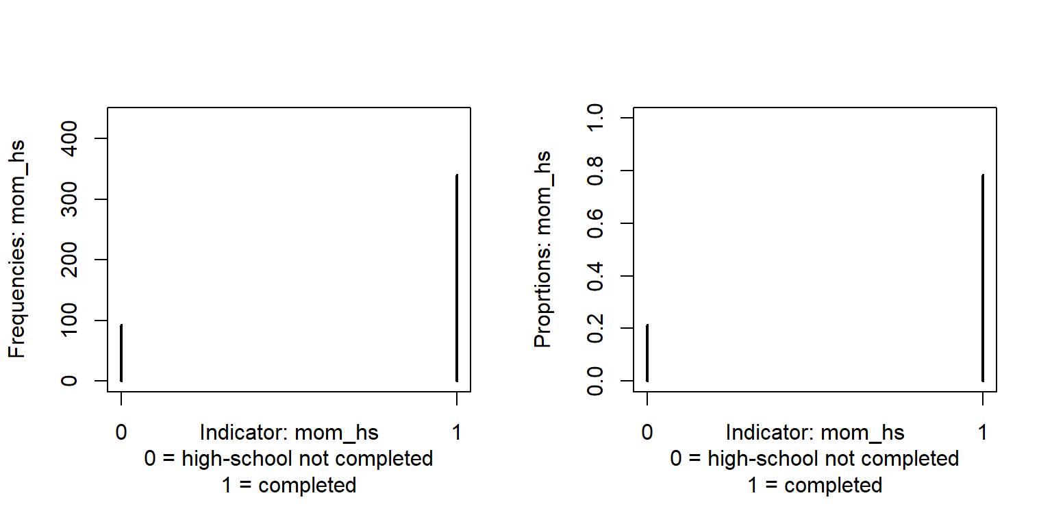

Code

table(d$mom_hs) # Frequency table


  0   1 
 93 341

Code

round(table(d$mom_hs)/length(d$mom_hs), 3)  # Proportions


    0     1 
0.214 0.786

Code

round(mean(d$mom_hs), 3)  # Mean indicator should be the same as proportion 1's

[1] 0.786

Estimating a difference between two means is the same as regressing on an indicator variable

Consider this model:

$y_i \sim N(\mu_i, \sigma)$
$\mu_i = b_0 + b_1D_i$, where $D_i$ is an indicator variable coded 0 or 1.

The interpretation of the coefficients is simple:

$b_0$ is the mean of $y_i$ for observations for which $D = 0$.
- That is, $b_0 = Mean(y_i | D = 0)$
$b_1$ is the difference in mean $y_i$ between observations for which $D = 1$ and $D = 0$.
- That is, $b_1 = Mean(y_i | D = 1) - Mean(y_i | D = 0)$,
- so, $Mean(y_i | D = 1) = b_0 + b_1$
$\sigma$ is the standard deviation of observations, assumed to be equal for observations in each group (homoscedasticity)

Here applied to outcome variable kid_score ($y_i$) and indicator variable moms_hs ($D_i$):

Code

# Note: stan_glm() is a method based on data simulation, the seed argument set 
# the random number generator
m1 <- stan_glm(kid_score ~ mom_hs, data = d, refresh = 0, seed = 123)
print(m1)

stan_glm
 family:       gaussian [identity]
 formula:      kid_score ~ mom_hs
 observations: 434
 predictors:   2
------
            Median MAD_SD
(Intercept) 77.5    2.0  
mom_hs      11.8    2.3  

Auxiliary parameter(s):
      Median MAD_SD
sigma 19.9    0.7  

------
* For help interpreting the printed output see ?print.stanreg
* For info on the priors used see ?prior_summary.stanreg

Code

posterior_interval(m1, prob = 0.95)

                2.5%    97.5%
(Intercept) 73.40918 81.54022
mom_hs       7.26764 16.36398
sigma       18.64532 21.28927

Interpretation: On average, kids to mothers who completed high-school had 12 points higher scores than kids to mothers who did not complete high-school. Our data is compatible with a difference in the population between about 7 - 16 points, given the assumptions of our statistical model (independent observations, normal distributions with equal standard deviations).

10.3 Categorical variables

Categorical variables code membership in categories for nominal scale variables. In the kidIQ data, the variable mom_work is a nominal variable coding the amount of work of mothers during their kid’s first three years. It is coded 1, 2, 3, and 4 for the four categories described above in the code book. This is a nominal scale value, although it can be discussed whether it also can be interpreted as an ordinal scale, from the least to the most amount of work during the first three years of child’s life (more information would be needed on the definition of the variable to decide this).

The categorical variable mom_work could be coded as three indicator variables, for example:

$D_2$ coded 1 if mom_work = 2 and 0 otherwise,
$D_3$ coded 1 if mom_work = 3 and 0 otherwise, and
$D_4$ coded 1 if mom_work = 4 and 0 otherwise.

The first category, mom_work = 1, would be implied for observations for which $D_2 = D_3 = D_4 = 0$. In general, a categorical variable with $k$ categories can be coded with $k-1$ indicator variables. However, in R it is possible to use a categorical variable (factor) to obtain the same thing. Here a boxplot of kid_score for each category of mom_work

Code

# Make mom_work a factor, and add labels (labels not needed, but helpful)
d$mom_work_f <- factor(d$mom_work, 
                  levels = c(1, 2, 3, 4),
                  labels = c("1_no", "2_only_y2_y3","3_part_y1", "4_full_y1"))
boxplot(d$kid_score ~ d$mom_work_f, xlab = "Categorical variable: mom_work",
        ylab = "Kids score on intelligence test", col = "lightblue")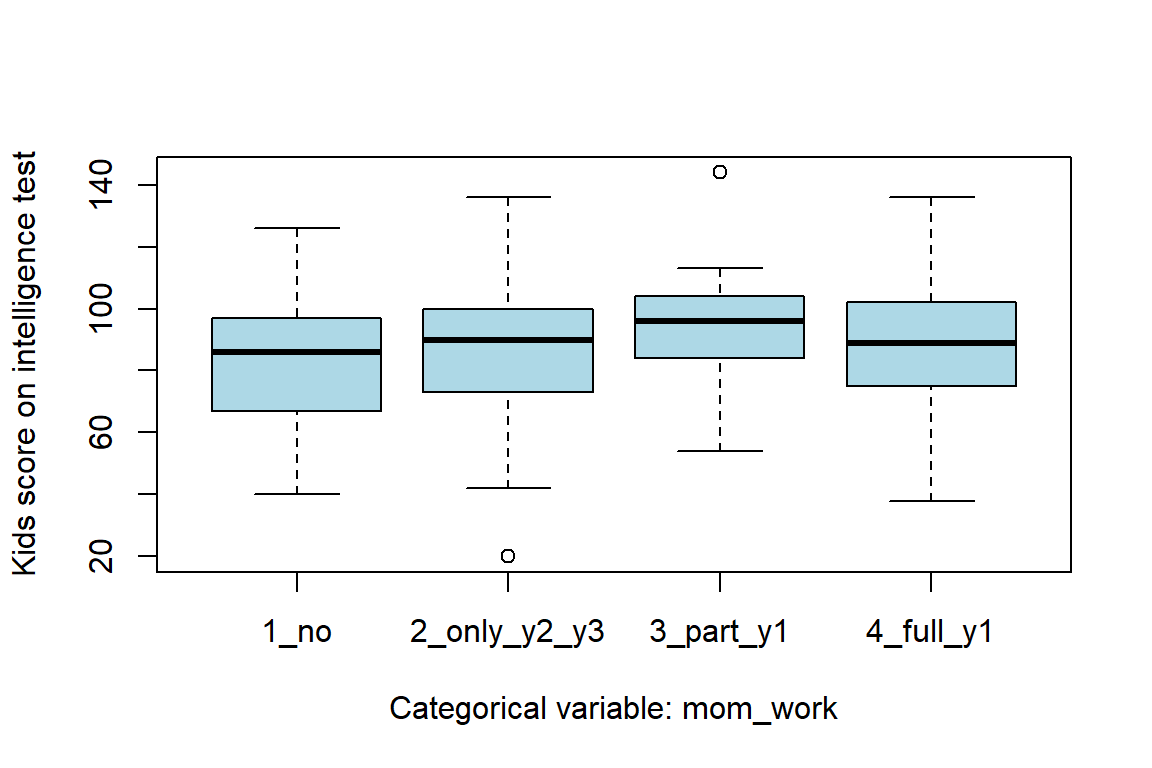

Estimating differences between several means is the same as regressing on a categorical variable

R will analyse a categorical variable (factor) with $k$ categories as an analysis with $k-1$ indicator variables. The analysis will estimate one regression coefficient for each category except the first category (reference). The regression coefficients refer to the mean difference between the group defined by the category and the group defined by the reference category. The intercept estimates the mean of the reference category.

Here an example predicting kid_score from mom_work using stan_glm():

Code

# Use factor, defined previous code block
m2 <- stan_glm(kid_score ~ mom_work_f, data = d, refresh = 0, seed = 123)
print(m2)

stan_glm
 family:       gaussian [identity]
 formula:      kid_score ~ mom_work_f
 observations: 434
 predictors:   4
------
                       Median MAD_SD
(Intercept)            82.1    2.3  
mom_work_f2_only_y2_y3  3.7    3.1  
mom_work_f3_part_y1    11.4    3.5  
mom_work_f4_full_y1     5.2    2.6  

Auxiliary parameter(s):
      Median MAD_SD
sigma 20.3    0.7  

------
* For help interpreting the printed output see ?print.stanreg
* For info on the priors used see ?prior_summary.stanreg

Code

posterior_interval(m2, prob = 0.95)

                             2.5%     97.5%
(Intercept)            77.4093836 86.486748
mom_work_f2_only_y2_y3 -2.3954141  9.963632
mom_work_f3_part_y1     4.3567994 18.604737
mom_work_f4_full_y1    -0.1811025 10.592623
sigma                  18.9977610 21.716944

The reference category (1: no work) had a mean of around 82 points. Categories 2, 3, and, 4 had higher scores the first category, about 4, 11, and 5 points, respectively.

You can change the reference category by redefining the factor:

Code

# Make 4: full-time work the reference category. 
d$mom_work_f <- factor(d$mom_work, 
                  levels = c(4, 1, 2, 3),
                  labels = c("4_full_y1", "1_no", "2_only_y2_y3","3_part_y1"))
m2 <- stan_glm(kid_score ~ mom_work_f, data = d, refresh = 0, seed = 123)
print(m2)

stan_glm
 family:       gaussian [identity]
 formula:      kid_score ~ mom_work_f
 observations: 434
 predictors:   4
------
                       Median MAD_SD
(Intercept)            87.2    1.4  
mom_work_f1_no         -5.2    2.8  
mom_work_f2_only_y2_y3 -1.4    2.5  
mom_work_f3_part_y1     6.3    3.1  

Auxiliary parameter(s):
      Median MAD_SD
sigma 20.2    0.7  

------
* For help interpreting the printed output see ?print.stanreg
* For info on the priors used see ?prior_summary.stanreg

The reference category (4: full time work) had a mean of around 87 points. Categories 1 and 2 had lower scores than category 4, whereas category 3 had higher scores.

10.4 One continous predictor

Estimating the relationship between Mothers IQ-score (mom_iq) and kid_score

Code

m3 <- stan_glm(kid_score ~ mom_iq, data = d, refresh = 0, seed = 123)
print(m3)

stan_glm
 family:       gaussian [identity]
 formula:      kid_score ~ mom_iq
 observations: 434
 predictors:   2
------
            Median MAD_SD
(Intercept) 25.8    5.9  
mom_iq       0.6    0.1  

Auxiliary parameter(s):
      Median MAD_SD
sigma 18.3    0.6  

------
* For help interpreting the printed output see ?print.stanreg
* For info on the priors used see ?prior_summary.stanreg

Plot data and model prediction

Code

# Scatter plot
plot(d$mom_iq, d$kid_score, 
     xlab = "Mother's IQ-score", 
     ylab = "Kid's score on IQ-related measure")
abline(m3$coefficients)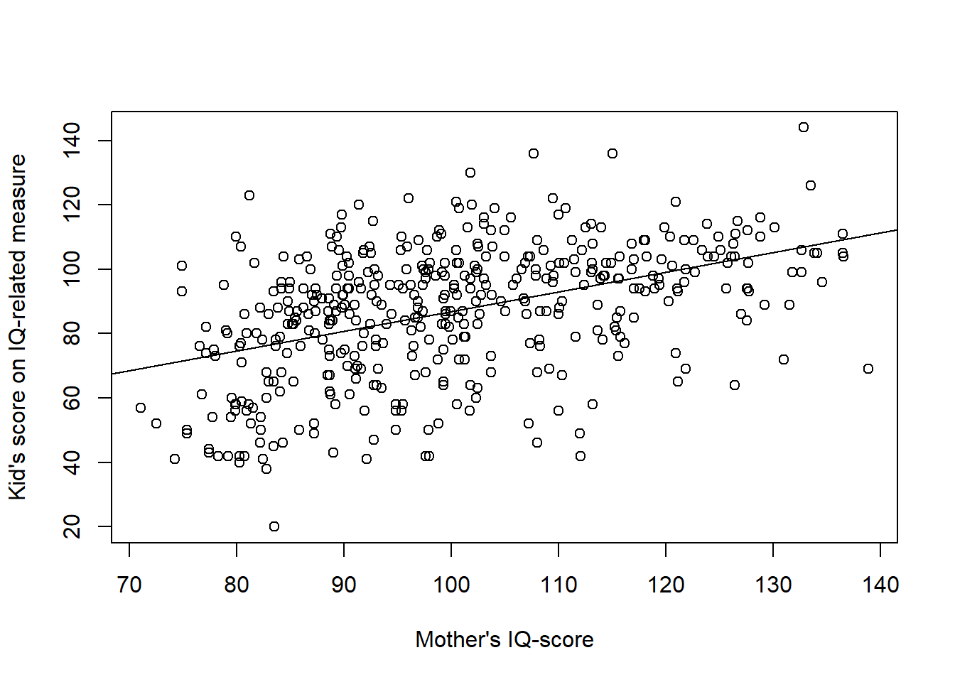

Centering of predictor to make intercept meaningful

In the model above, the intercept = 25.81 is not meaningful as it refer to the kid_score of a kid to a mother with an IQ-score = 0 (an impossible value). Centering the predictor:

d$mom_iq_centered <- d$mom_iq - mean(d$mom_iq)

make the intercept meaningful: It is the kid_score of a kid to a mother with a mean IQ-score. Note that the slope remains the same.

Code

# Center the predictor variable
d$mom_iq_centered <- d$mom_iq - mean(d$mom_iq)

# Fit model
m3center <- stan_glm(kid_score ~ d$mom_iq_centered, 
                     data = d, refresh = 0, seed = 123)
print(m3center)

stan_glm
 family:       gaussian [identity]
 formula:      kid_score ~ d$mom_iq_centered
 observations: 434
 predictors:   2
------
                  Median MAD_SD
(Intercept)       86.8    0.9  
d$mom_iq_centered  0.6    0.1  

Auxiliary parameter(s):
      Median MAD_SD
sigma 18.3    0.6  

------
* For help interpreting the printed output see ?print.stanreg
* For info on the priors used see ?prior_summary.stanreg

Code

# Scatter plot
plot(d$mom_iq_centered, d$kid_score, 
     xlab = "Mother's IQ-score, centered around mean(IQ-score)", 
     ylab = "Kid's score on IQ-related measure")
abline(m3center$coefficients)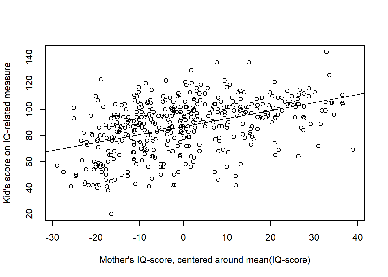

10.5 Advanced: Parameterization

A model can often be written in several ways, with different sets of parameters. The models, or parameterizations, are mathematically equivalent, but one parameterization may be more useful than another.

As an example, consider these two parameterizations of the same model:

m1:
- $y_i \sim N(\mu_i, \sigma)$
- $\mu_i = b_0 + b_1D_i$, where $D_i$ is an indicator variable coded 0 or 1.
m1b:
- $y_i \sim N(\mu_i, \sigma)$
- $\mu_i = b_0D_{1i} + b_1D_{2i}$, where
  - $D_{1}$ is an indicator variable where 1 means that the mother did not complete high school,
  - $D_{2}$ is an indicator variable where 1 means that the mother did complete high school.

In parameterization m1, $b_1$ refer to a difference between means, whereas in m1b, $b_1$ refer to the mean of observations for which $D = 1$. In both parameterizations, $b_0$ refer to the mean of observations for which $D = 0$.

If your goal is to estimate group means rather than differences between means,
parameterization m1b may be your choice. Note that m1b still assume equal standard deviations. (If you don’t like this assumption, then just fit an intercept-only model separately to each group of kids.)

Here the two versions of the model are fitted using glm():

Code

d$mom_hs0 <- 1 * (d$mom_hs == 0)  # New indicator variable

# Model with intercept and one indicators
m1_lm <- glm(kid_score ~ mom_hs, data = d)

# Model with no intercept and two indicators
m1b_lm <- glm(kid_score ~ 0 + mom_hs0 + mom_hs, data = d)

# Model outputs
summary(m1_lm)


Call:
glm(formula = kid_score ~ mom_hs, data = d)

Coefficients:
            Estimate Std. Error t value Pr(>|t|)    
(Intercept)   77.548      2.059  37.670  < 2e-16 ***
mom_hs        11.771      2.322   5.069 5.96e-07 ***
---
Signif. codes:  0 '***' 0.001 '**' 0.01 '*' 0.05 '.' 0.1 ' ' 1

(Dispersion parameter for gaussian family taken to be 394.1231)

    Null deviance: 180386  on 433  degrees of freedom
Residual deviance: 170261  on 432  degrees of freedom
AIC: 3829.5

Number of Fisher Scoring iterations: 2

Code

summary(m1b_lm)


Call:
glm(formula = kid_score ~ 0 + mom_hs0 + mom_hs, data = d)

Coefficients:
        Estimate Std. Error t value Pr(>|t|)    
mom_hs0   77.548      2.059   37.67   <2e-16 ***
mom_hs    89.320      1.075   83.08   <2e-16 ***
---
Signif. codes:  0 '***' 0.001 '**' 0.01 '*' 0.05 '.' 0.1 ' ' 1

(Dispersion parameter for gaussian family taken to be 394.1231)

    Null deviance: 3450038  on 434  degrees of freedom
Residual deviance:  170261  on 432  degrees of freedom
AIC: 3829.5

Number of Fisher Scoring iterations: 2

You may of course do the same thing with stan_glm(). But it may not be necessary, as you can use it’s parameter estimates to derive new parameters. Here an illustration, using parameter estimates from model m1:

$y_i \sim N(\mu_i, \sigma)$
$\mu_i = b_0 + b_1D_i$,

to derive point estimate and 95 % confidence interval for the mean of the group $D = 1$, that is, $b_0 + b_1$, for the kidIQ data.

Samples from the posterior:

Code

# Fit model using glm_stan()
m1 <- stan_glm(kid_score ~ mom_hs, data = d, refresh = 0, seed = 123)

# Save samples from the posterior distribution
samples <- as.data.frame(m1)
names(samples) <- c("b0", "b1", "sigma")  # rename column names

# Derive new estimate: b0 + b1
samples$mean_g1 <- samples$b0 + samples$b1
head(samples)

        b0        b1    sigma  mean_g1
1 79.26794 10.223293 19.09675 89.49123
2 80.57249 10.290838 19.24931 90.86332
3 79.01779  9.521749 19.85170 88.53954
4 76.58362 13.120297 20.32644 89.70392
5 77.75065 12.179655 19.70027 89.93030
6 77.85677 12.065890 19.95251 89.92266

Estimates from glm_stan():

Code

# median and 95 % CI for group 1 (mom_hs = 1)
g1posterior <- quantile(samples$mean_g1, probs = c(0.025, 0.5, 0.975))
g1posterior

    2.5%      50%    97.5% 
87.21719 89.30087 91.43292

Code

# Plot posterior, with point estimate and 95 % CI
plot(density(samples$mean_g), main = "", 
     xlab = "Estimated mean IQ-score for kids to \nmothers with completed high-school", 
     ylab = "Posterior probabbility")
lines(x = c(g1posterior[1], g1posterior[3]), y = c(0.01, 0.01),
      col = "blue")
points(g1posterior[2], 0.01, pch = 21, bg = "lightblue")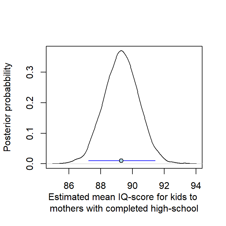

The estimated interval is almost identical to the estimates of parameterization m1b using glm() (or stan_glm())

Estimates from glm(kid_score ~ 0 + mom_hs0 + mom_hs, data = d)

Code

m1b <- glm(glm(kid_score ~ 0 + mom_hs0 + mom_hs, data = d))
point_est <- m1b$coefficients[2]
names(point_est) <- ""
ci95lo <- confint(m1b)[2, 1]
ci95hi <- confint(m1b)[2, 2]
m1b_estimates <- c(ci95lo = ci95lo, point_est = point_est, ci95hi = ci95hi)
round(m1b_estimates, 3)

   ci95lo point_est    ci95hi 
   87.213    89.320    91.427

A similar strategy can be used with categorical variables: by excluding the intercept, regression coefficients refer to mean values for each category. Here illustrated using the four-category variable mom_work as predictor and kid_score as outcome variable, using stan_glm() and lm():

Code

# Model with no intercept yields estimates of means for each category
m2b <- stan_glm(kid_score ~ 0 + mom_work_f, data = d, refresh = 0, seed = 123)
print(m2b)

stan_glm
 family:       gaussian [identity]
 formula:      kid_score ~ 0 + mom_work_f
 observations: 434
 predictors:   4
------
                       Median MAD_SD
mom_work_f4_full_y1    87.2    1.5  
mom_work_f1_no         81.9    2.2  
mom_work_f2_only_y2_y3 85.9    2.0  
mom_work_f3_part_y1    93.5    2.6  

Auxiliary parameter(s):
      Median MAD_SD
sigma 20.2    0.7  

------
* For help interpreting the printed output see ?print.stanreg
* For info on the priors used see ?prior_summary.stanreg

Code

m2b_lm <- lm(kid_score ~ 0 + mom_work_f, data = d)
summary(m2b_lm)


Call:
lm(formula = kid_score ~ 0 + mom_work_f, data = d)

Residuals:
   Min     1Q Median     3Q    Max 
-65.85 -12.85   2.79  14.15  50.50 

Coefficients:
                       Estimate Std. Error t value Pr(>|t|)    
mom_work_f4_full_y1      87.210      1.413   61.72   <2e-16 ***
mom_work_f1_no           82.000      2.305   35.57   <2e-16 ***
mom_work_f2_only_y2_y3   85.854      2.065   41.58   <2e-16 ***
mom_work_f3_part_y1      93.500      2.703   34.59   <2e-16 ***
---
Signif. codes:  0 '***' 0.001 '**' 0.01 '*' 0.05 '.' 0.1 ' ' 1

Residual standard error: 20.23 on 430 degrees of freedom
Multiple R-squared:  0.949, Adjusted R-squared:  0.9485 
F-statistic:  2000 on 4 and 430 DF,  p-value: < 2.2e-16

Compare these estimates to the the sample means for each category:

Code

aggregate(list(kid_score = d$kid_score), list(mom_work = d$mom_work_f), mean)

      mom_work kid_score
1    4_full_y1  87.20976
2         1_no  82.00000
3 2_only_y2_y3  85.85417
4    3_part_y1  93.50000

Practice

The practice problems are labeled Easy (E), Medium (M), and Hard (H), (as in McElreath (2020)).

Easy

10E1. Load the data in the file earnings.txt. It is data from a survey conducted 1990. This data set is used by Gelman et al. (2021) at several places. Please find a code book for this data set below the Practice section.

Weight is given in pounds. Transform it to kilograms, and estimate average weight in the population using regression (intercept-only regression), report point estimate and 90 % compatibility interval.
Make a histogram overlaid with a kernel density estimate of the observed weight [kg], and discuss in relation to assumptions of your model.

10E2. Continue on 10E1, but now estimate the difference in weight between males and females by regressing on an indicator variable. Report point estimate and 90 % compatibility interval.

10E3. Continue on 10E1, but now estimate the difference in weight between groups defined by ethnicity (Blacks, Whites, Hispanics, Other):

With Blacks s reference category.
With Whites as reference category.

10E4. Below is estimated coefficients from glm(). What does the coefficients refer to?

Code

m <- read.table("datasets/earnings.txt", header = TRUE, sep = ",")
m$weight_kg <- m$weight * 0.45359237
m$ethnicity_f <- factor(m$ethnicity)
fit <- glm(weight_kg ~ 0 + ethnicity_f, data = m)
fit


Call:  glm(formula = weight_kg ~ 0 + ethnicity_f, data = m)

Coefficients:
   ethnicity_fBlack  ethnicity_fHispanic     ethnicity_fOther  
              72.63                68.96                64.91  
   ethnicity_fWhite  
              70.97  

Degrees of Freedom: 1789 Total (i.e. Null);  1785 Residual
  (27 observations deleted due to missingness)
Null Deviance:      9434000 
Residual Deviance: 438600   AIC: 14930

Medium

10M1. Below a scatter plot of the relationship between weight [kg] and age [years] from the earnings.txt data (used above in 10E1). The smooth function was added using the loess() function in R.

Based on the plot and the red line, would linear regression seem useful to estimate the relationship?
If you could add one additional predictor to reduce the variability around the regression line, which one would you suggest?

Code

m <- read.table("datasets/earnings.txt", header = TRUE, sep = ",")
m$weight_kg <- m$weight * 0.45359237
plot(m$age, m$weight_kg, xlab = "Age [years]", ylab = "Weight [kg]")

# Fit loess() line // lowess() did not work well here for some reason
loess_fit <- loess(weight_kg ~ age, data = m)
dd <- data.frame(age = seq(18, 90, length.out = 100))
predicted <- predict(loess_fit, newdata = dd)
lines(dd$age, predicted, col = "red", lwd = 3, lty = 3)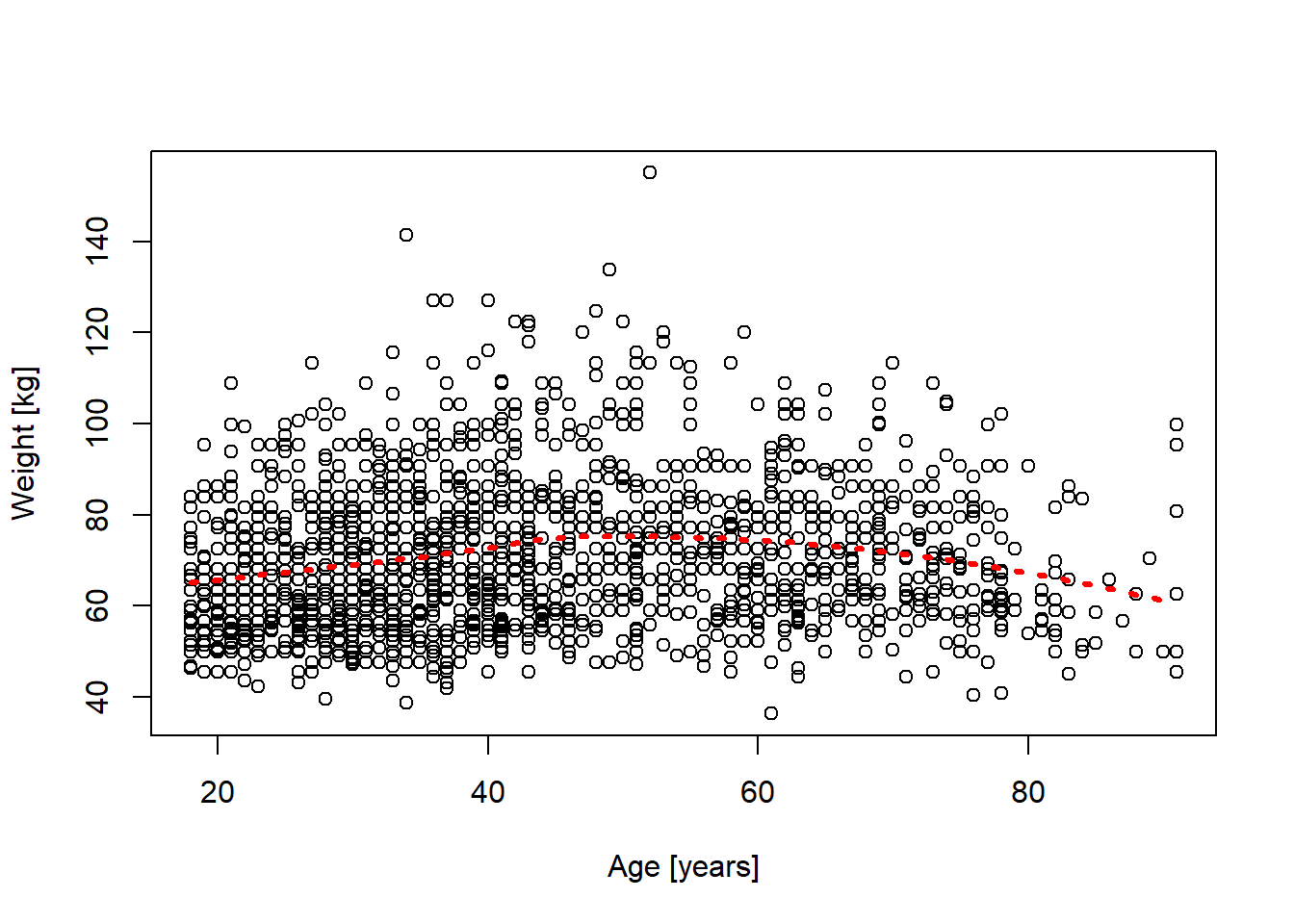

10M2. Below a scatter plot of the relationship between weight [kg] and age [years] for males < 50 years old. The line was fitted using linear regression (glm(weight_kg ~ age)).

Estimate by eye the intercept and slope of regression line.
The intercept makes little sense (why?), how would you fix that?

Code

mm <- m[m$male == 1 & (m$age < 50), c("weight_kg", "age")]
plot(mm$age, mm$weight_kg, xlab = "Age [years]", ylab = "Weight [kg]")
mmfit <- glm(weight_kg ~ age, data = mm)
abline(mmfit, col = "blue")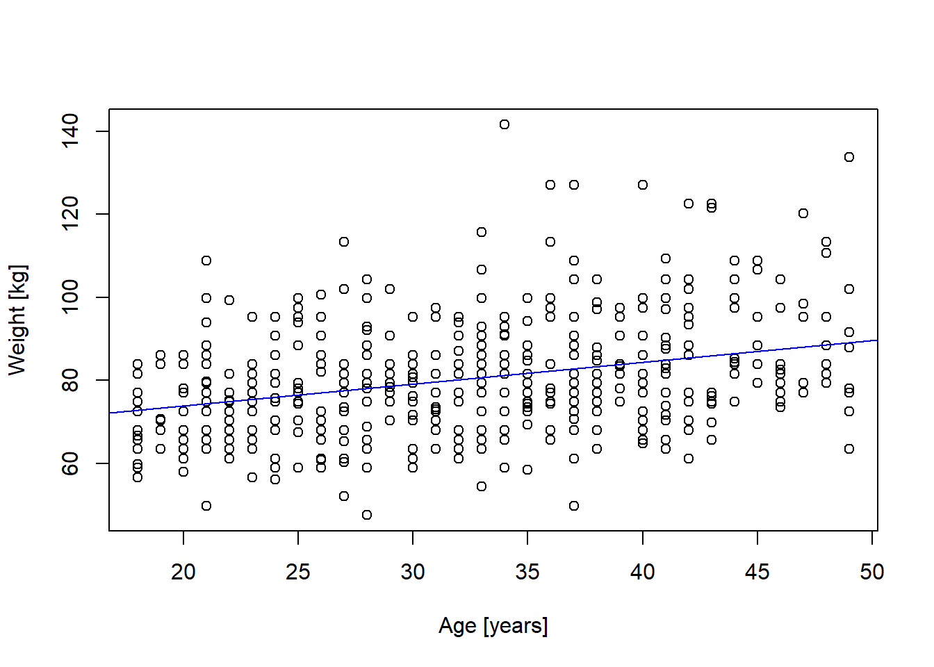

10M3. Below is a summary of a regression model for the data in 10M2, i.e., for men < 50 years old. This time with the predictor centered at 20 years and expressed in decades: $age20dec = (age - 20)/10$.

Given an approximate 95 % confidence around the regression coefficient for the age variable
In one sentence, describe how weight and age are related according to the regression model in terms of weight differences per decade, with reference to both point and interval estimate.
Reexpress (b), but now assume a causal relationship between age and weight.
Would you assess the size of the age-effect on weight to be reasonable? Discuss.

Code

mm$age20dec <- (mm$age - 20)/10
mmfit <- glm(weight_kg ~ age20dec, data = mm)
summary(mmfit)


Call:
glm(formula = weight_kg ~ age20dec, data = mm)

Coefficients:
            Estimate Std. Error t value Pr(>|t|)    
(Intercept)  73.9696     1.0516   70.34  < 2e-16 ***
age20dec      5.2100     0.7127    7.31 1.15e-12 ***
---
Signif. codes:  0 '***' 0.001 '**' 0.01 '*' 0.05 '.' 0.1 ' ' 1

(Dispersion parameter for gaussian family taken to be 173.4478)

    Null deviance: 91309  on 474  degrees of freedom
Residual deviance: 82041  on 473  degrees of freedom
AIC: 3801

Number of Fisher Scoring iterations: 2

10M4. I wanted to explore whether smokers have lower weight than non-smokers. I used the data from above (earnings.txt, full sample) and used linear regression to fit this model:

\[weight_i \sim Normal(\mu_i, \sigma) \\ \mu_i= b_0 + b_1 smoke_i \]

where $weight$ is in kg and $smoke$ is an indicator variable coded 1 if current smoker and 0 if not.

Below is a summary of the regression result. This time I used stan_glm() from the rstanarm package.

Explain the meaning of the three estimated parameter values: $b_0, b_1, \sigma$.
Summarize the result in a single sentence with respect to the hypothesis that smokers have lower weight than non-smokers, refer to both point and interval estimates of the coefficient for smoke. Provide two versions: (1) In terms of differences between groups, and (2) in terms of causal effect.
The result was in the expected direction: smokers had lower weight than non-smokers in this sample. Still, the causal interpretation (b) may still be wrong. Discuss potential confounders (some available in the data set, see code book below).

Code

# Indicator-coded smoking variable: 1 if smoker (<7 cigs a week), 0 if not.  
# smokenow in the original data set was defined as 1 for more than 7 cigs per 
# week, 2 if not.
m$smoke <- ifelse(m$smokenow == 1, 1, 0)

# Fit model, note: refresh = 0 suppresses output to the console, not needed
smokefit <- rstanarm::stan_glm(weight_kg ~ smoke, data = m, refresh = 0)
print(smokefit)

stan_glm
 family:       gaussian [identity]
 formula:      weight_kg ~ smoke
 observations: 1788
 predictors:   2
------
            Median MAD_SD
(Intercept) 71.4    0.4  
smoke       -2.0    0.9  

Auxiliary parameter(s):
      Median MAD_SD
sigma 15.7    0.3  

------
* For help interpreting the printed output see ?print.stanreg
* For info on the priors used see ?prior_summary.stanreg

Hard

10H1. This exercise is a version of Exercise 7.7 from Gelman et al. (2021):

Draw 100 values of the predictor x from a uniform distribution between 0 and 50. Then simulate 100 observations ($y_i$, where $i = 1, 2, ..., 100$) from this model:

$y_i \sim Normal(\mu_i = 2 + 5x_i, \sigma = 10)$

Save x and y in a data frame called fake and fit the model

stan_glm(y ~ x, data = fake) (or use glm() instead).

Plot data and regression line. Add regression equation to the plot.
Are the estimated coefficients close to the assumed true values? Discuss a way of defining “close” in this context.

10H2. This exercise is a version of Exercise 7.8 from Gelman et al. (2021):

Repeat the simulation in 10H1 a thousand times (omit plotting). Check that the coefficient estimates ($b_0, b_1, \sigma$) are centered around the true parameter values.

Data set earnings.txt

The data set is from a survey on “Work, family, and well-being in the United States” conducted in 1990. Gelman et al. use it as several places, for example, pp. 84-85 and 189-195. The data set provided by Gelman et al. is a selection of variables from the original study, and they have excluded respondents with missing data on height or earnings (see footnote 4, page 84). I managed to reconstruct a code book of the variables in the data set from the surveys code book, available at the Gelman et al’s web site.

Code book

height – Height [inches]
weight – Wight [pounds]
male – Sex: male = 1, female = 0
earn – Personal income in 1989 before taxes [USD]
earnk – Personal income in 1989 before taxes [kUSD]
ethnicity – Black, Hispanic, White, or Other
education – Highest grade or year of school:
- 0 None
- 1-8 Elementary school
- 9-12 High school
- 14-16 College
- 17 Some graduate school
- 18 Graduate or professional degree
- 99 Don’t know
mother_education – Highest grade or year of school mother. Code as for education.
father_education – Highest grade or year of school father. Code as for education.
walk – Frequency of talking a walk, including walking to work, train station, etc.
- 1 Never
- 2 Once a month or less
- 3 About twice a week
- 4 About once a week
- 5 Twice a week
- 6 Three times a week
- 7 More than 3 times a week
- 8 Every day
exercise – Frequency of strenuous exercising. A bit unclear how this was measured, but I guess it was a categorical scale from rarely (1) to often (7).
smokenow – Smoke 7 or more cigarettes a week. 1 = yes, 2 = no.
tense – On how many of the past 7 days have you felt tense or anxious? 0-7.
angry – On how many of the past 7 days have you felt angry?
age – Age [years]

Follow this link to find data Save (Ctrl+S on a PC) to download as text file

(Session Info)

Code

sessionInfo()

R version 4.4.2 (2024-10-31 ucrt)
Platform: x86_64-w64-mingw32/x64
Running under: Windows 11 x64 (build 26100)

Matrix products: default


locale:
[1] LC_COLLATE=Swedish_Sweden.utf8  LC_CTYPE=Swedish_Sweden.utf8   
[3] LC_MONETARY=Swedish_Sweden.utf8 LC_NUMERIC=C                   
[5] LC_TIME=Swedish_Sweden.utf8    

time zone: Europe/Stockholm
tzcode source: internal

attached base packages:
[1] stats     graphics  grDevices utils     datasets  methods   base     

other attached packages:
[1] rstanarm_2.32.1 Rcpp_1.0.14    

loaded via a namespace (and not attached):
 [1] tidyselect_1.2.1     dplyr_1.1.4          farver_2.1.2        
 [4] loo_2.8.0            fastmap_1.2.0        tensorA_0.36.2.1    
 [7] shinystan_2.6.0      promises_1.3.3       shinyjs_2.1.0       
[10] digest_0.6.37        mime_0.13            lifecycle_1.0.4     
[13] StanHeaders_2.32.10  survival_3.7-0       magrittr_2.0.3      
[16] posterior_1.6.1      compiler_4.4.2       rlang_1.1.6         
[19] tools_4.4.2          igraph_2.1.4         yaml_2.3.10         
[22] knitr_1.50           htmlwidgets_1.6.4    pkgbuild_1.4.8      
[25] curl_6.4.0           plyr_1.8.9           RColorBrewer_1.1-3  
[28] dygraphs_1.1.1.6     abind_1.4-8          miniUI_0.1.2        
[31] grid_4.4.2           stats4_4.4.2         xts_0.14.1          
[34] xtable_1.8-4         inline_0.3.21        ggplot2_3.5.2       
[37] scales_1.4.0         gtools_3.9.5         MASS_7.3-61         
[40] cli_3.6.5            rmarkdown_2.29       reformulas_0.4.1    
[43] generics_0.1.4       RcppParallel_5.1.10  rstudioapi_0.17.1   
[46] reshape2_1.4.4       minqa_1.2.8          rstan_2.32.7        
[49] stringr_1.5.1        shinythemes_1.2.0    splines_4.4.2       
[52] bayesplot_1.13.0     parallel_4.4.2       matrixStats_1.5.0   
[55] base64enc_0.1-3      vctrs_0.6.5          V8_6.0.4            
[58] boot_1.3-31          Matrix_1.7-1         jsonlite_2.0.0      
[61] crosstalk_1.2.1      glue_1.8.0           nloptr_2.2.1        
[64] codetools_0.2-20     distributional_0.5.0 DT_0.33             
[67] stringi_1.8.7        gtable_0.3.6         later_1.4.2         
[70] QuickJSR_1.8.0       lme4_1.1-37          tibble_3.3.0        
[73] colourpicker_1.3.0   pillar_1.10.2        htmltools_0.5.8.1   
[76] R6_2.6.1             Rdpack_2.6.4         evaluate_1.0.3      
[79] shiny_1.11.1         lattice_0.22-6       markdown_2.0        
[82] rbibutils_2.3        backports_1.5.0      threejs_0.3.4       
[85] httpuv_1.6.16        rstantools_2.4.0     gridExtra_2.3       
[88] nlme_3.1-166         checkmate_2.3.2      xfun_0.52           
[91] zoo_1.8-14           pkgconfig_2.0.3