11 M: Broken Experiments and Quasi-experiments

Load R-libraries

Code

library(dagitty) # R implementation of http://www.dagitty.net

Warning: package 'dagitty' was built under R version 4.4.3

Topics

Non-compliance and missing data: Why they may introduce bias in randomized experiments (DAGs are helpful to illustrate)
Complier types
- Compliers
- Always takers
- Never takers
- Defiers
Broken experiments: Analytic approaches.
- Non-compliance
  - As treated (AT) analysis
  - Per protocol (PP) analysis
  - Intention to treat (ITT) analysis
  - Treatment effect bounding
- Missing data
  - Complete cases analysis. Understand risk of bias.
  - Last observation carried forward. Understand risk of bias.
  - Mean or regression based imputation of single values. Understand risk of bias.
  - (Multiple imputation: a better alternative but not covered in this course)

Theoretical articles to read:

Gelman et al. (2021), chapter 18, sections 18.3 - 18.6. Understand SATE and PATE, and tables 18.3-5. (For the interested reader, Chapter 17 of Gelman et al’s book has a nice discussion of missing data, however, this chapter is not part of the course.)
Sagarin et al. (2014), Focus on: ITT, AT and PP analysis (pp. 317 320, 327 328), and the four patterns of compliance (p. 321).
Rohrer (2018) is an excellent introduction to DAGs.

11.1 Randomized experiment: How can I loose?

The randomized experiment is often labeled the “Gold standard” of causal inference. A bit undeservedly if you ask me:

Single-unit causal effects still unknown. Remember: SATE (or PATE) close to zero does not imply absence of single-unit causal effects; moderate or small SATE (or PATE) consistent with substantial single-unit causal effect. Single-unit causal effects can only be inferred given strong assumptions. For example, assumptions about normally distributed single-unit causal effects would imply that the average causal effect is representative of the typical individual, or the assumption of constant treatment effect (West & Thoemmes (2010), p. 23) would imply that the average causal effect is representative of every individual (unrealistic for most behavioral science phenomena, people react differently to stimuli and treatments).
Non-compliance may introduce systematic error (as discussed below), and internal validity issues, as well as issues with external validity (results generalizes only to compliers).
Drop out may introduce systematic error (as discussed below), and internal validity issues, as well as issues with external validity (results generalizes only to non-drop outs).
Construct validity issues: What was the mechanism of the observed effect? Threats include Placebo and Hawthorne effects (e.g., Gelman et al. (2021), p. 354).
Randomization error (remedy: large n). May lead to discrepancy between SATE and prima-facie estimate, due to randomization errors and thereby issues with internal validity.
Sampling error (remedy: large n). May lead to discrepancy between SATE and PATE, due to sampling error and thereby issues with external validity.

To be fair, some of the above applies also to within-subject experiments, including
Single-N designs (my “Gold standard”).

Below I will use Directed Acyclical Graphs (DAGs) to illustrate how confounding may cause problems even in large randomized experiments with non-compliance or attrition.

11.2 Non-compliance

Problem: Confounding by unmeasured variable causing both treatment compliance and outcome.

Randomized experiment

Code

library(dagitty) # R version of http://www.dagitty.net

randomized_exp <- dagitty( "dag {
   Random -> Treatment
   Treatment -> Outcome
   Z -> Outcome
}")

coordinates(randomized_exp) <- list(
  x = c(Random = 1, Treatment = 2, Z = 2.5, Outcome = 3),
  y = c(Random = 2, Treatment = 2, Z = 1.5, Outcome = 2))

plot(randomized_exp)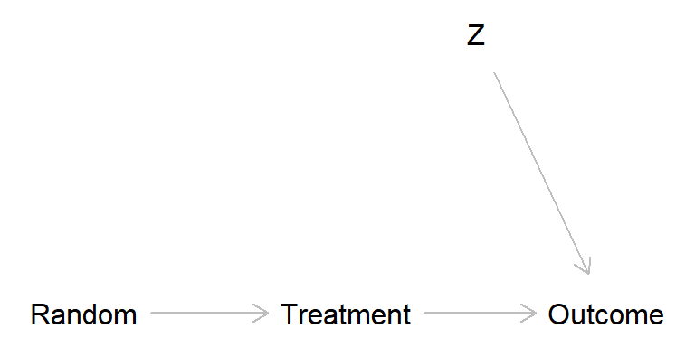

Broken randomized experiment (treatment has a causal effect)

Code

broken_exp <- dagitty( "dag {
   Random -> Treatment
   Treatment -> Outcome
   Z -> Treatment -> Outcome
   Z -> Outcome
}")

coordinates(broken_exp) <- list(
  x = c(Random = 1, Treatment = 2, Z = 2.5, Outcome = 3),
  y = c(Random = 2, Treatment = 2, Z = 1.5, Outcome = 2))

plot(broken_exp)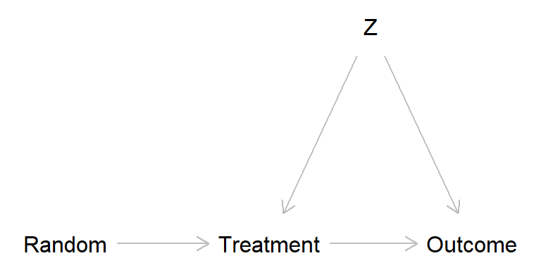

Broken randomized experiment (treatment has no causal effect)

Code

broken_exp2 <- dagitty( "dag {
   Random -> Treatment
   Z -> Treatment
   Z -> Outcome
}")

coordinates(broken_exp2) <- list(
  x = c(Random = 1, Treatment = 2, Z = 2.5, Outcome = 3),
  y = c(Random = 2, Treatment = 2, Z = 1.5, Outcome = 2))

plot(broken_exp2)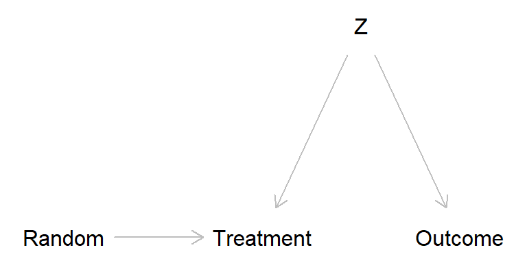

The problem is that \(Z\) in the broken experiment scenarios may introduce bias. One way to think about this is offered by the potential outcome perspective, from which we may define four “causal types”. Think of an experiment in which kids are randomly assigned to “music lesson” (treatment) or “no music lessons” (control), cf. Schellenberg (2004).

Compliers will do as we say: if assigned to “music lesson” they will take music lessons, if assigned to “no music lessons” they will not take music lessons.
Always-takers will always take the treatment: if assigned to “music lesson” they will take music lessons, if assigned to “no music lessons” they will nevertheless take music lessons.
Never-takers will never take the treatment: if assigned to “music lesson” they will not take music lessons, and same if they were assigned to “no music lessons”.
Defiers will never do as we say: if assigned to “music lesson” they will not take music lessons, if assigned to “no music lessons” they will take music lessons.

We usually assume that there are no defiers. Sometimes it is also possible to assume no always takers, if, for instance, we are administrating the music lessons we may make sure to only let in those who were assigned to treatment (but you never know, maybe an always-taker would buy similar music lessons from somewhere else).

It might be that the possible confounder \(Z\) may lead to unbalanced groups, for instance, \(Z\) might be socioeconomic status (SES), and maybe there are more never-takers among people with low compared to high SES. This may lead to lower SES among the non-treated than the treated, and this may look as an effect if treatment on the outcome. In Schellenberg (2004), the outcome was IQ scores, a variable that probably is related to SES.

11.3 Analytic approaches to non-compliance

Sagarin et al. (2014)

Intention-to-treat
As-treated
Per-protocol
Instrumental variable (not covered in this course)
Dose-response estimation (not covered in this course)
Propensity score analysis (not covered in this course)
Treatment effect bounding (briefly exemplified below)

Simple example:

Randomized experiment, 500 to Control group (do nothing), 500 to Experimental group (participate in training program).
Non-compliance: 100 participants in the treatment group did not take the treatment, and those were at high risk of mortality for other reasons (confounder Z).

Data

	Survived	Dead	Row sum
Control	450	50	500
Treatment	380	20	400
Control non-complier	80	20	100 (100 non-compliers, assigned to treatment)
Column sum	910	90	1000

Intention-to-treat

	Survived	Dead	Row sum
Control	450	50	500
Treatment	380 + 80	20 + 20	500 (400 + 100 non-compliers)
Column sum	910	90	1000

Code

# Relative risk and risk difference Control vs. Treated
RD <- c(RD = (50/500) - (40/500))
RR <- c(RR = (50/500) / (40/500))
round(c(RR, RD), 3)

  RR   RD 
1.25 0.02

As-treated analysis: Risk mortality in Control group vs. Treatment group

	Survived	Dead	Row sum
Control	450 + 80	50 + 20	600 (500 + 100 non-compliers)
Treatment	380	20	400
Column sum	910	90	1000

Code

# Relative risk and risk difference Control vs. Treated
RD <- c(RD = (70/600) - (20/400))
RR <- c(RR = (70/600) / (20/400))
round(c(RR, RD), 3)

   RR    RD 
2.333 0.067

Per-protocol analysis: Risk mortality in Control group vs. Treatment group

	Survived	Dead	Row sum
Control	450	50	500
Treatment	380	20	400
Column sum	830	70	900

Code

# Relative risk and risk difference Control vs. Treated
RD <- c(RD = (50/500) - (20/400))
RR <- c(RR = (50/500) / (20/400))
round(c(RR, RD), 3)

  RR   RD 
2.00 0.05

Hypotetical Data 1 (best case)
Assuming that all non-compliers (never-takers) would have survived had they taken the treatment

	Survived	Dead	Row sum
Control	450	50	500
Treatment	380 + 100	20	500 (400 + 100 surviving never-takers)
Column sum	930	70	1000

Upper bound: Risk mortality in Control group vs. Treatment group

Code

# Relative risk and risk difference Control vs. Treated
RDhi <- c(RDhi = (50/500) - (20/500))
RRhi <- c(RRhi = (50/500) / (20/500))
round(c(RRhi, RDhi), 3)

RRhi RDhi 
2.50 0.06

Hypotetical Data 2 (worst case)
Assuming that all never-takers would have died had they taken the treatment

	Survived	Dead	Row sum
Control	450	50	500
Treatment	380	20 + 100	500 (400 + 100 non-surviving never takers)
Column sum	830	170	1000

Lower bound: Risk mortality in Control group vs. Treatment group

Code

# Relative risk and risk difference Control vs. Treated
RDlo <- c(RDlo = (50/500) - (120/500))
RRlo <- c(RRlo = (50/500) / (120/500))
round(c(RRlo, RDlo), 3)

  RRlo   RDlo 
 0.417 -0.140

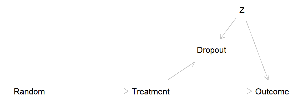
11.4 Missing data

Missing data may lead to similar problem as non-compliance, through adjusting for a collider variable and thereby introducing bias (often called attrition bias).

Classification of missing data:

Missingness completely at random (MCAR). The best scenario, probability of missingness is the same for all study units regardless of background variables. No bias related to missingness.
Missingness at random (MAR). The second best scenario: Probability of missingness depend only on observed variables, missing cases can be excluded if these observed variables are adjusted for.
Missingness not at random (MNAR). The worst scenario. Missingness related to unobserved variables, potentially inducing bias in causal effect estimates.

Common methods for dealing with missing data in randomized experiments (and elsewhere):

Complete cases. Analyse only cases for which there is no missing data on the outcome variable. If the experiment involve measures before and after treatment, this would require data on both. May lead to bias if missingness is not random, but is related to unmeasured confounders and treatment.
Last value carried forward. A common method, where missing data after treatment (“lost to follow up”) is replaced (imputed) with the before treatment measure. May lead to bias if missingness is not random, but related to unmeasured confounders or to treatment.
Mean imputation. Imputation of the mean of of the observed values for variable with missing data. May lead to an underestimation of the variable’s variance.
Predicted value Impute predicted value based on a regression analysis of participants with full data sets. Similar problem as mean imputation.
(Advanced methods, e.g., multiple imputation. not covered by this course. Generally viewed as superior to the above methods)

For more on missing data, see Gelman et al. (2021) Chapter 17, sections 3-6 (discussed further in the Statistics course).

Simple simulation of how missing data may introduce bias

This DAG show a scenario with no treatment effect and drop out related to a covariate Z, leading to attrition bias.

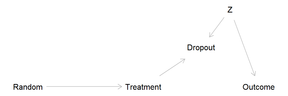
Here a simulation of this scenario.

Code

set.seed(999)

## Generate treatment and covariate variables
n <- 400  # Total sample size
rand <- sample(c(0, 1), size = n, replace = TRUE)  # Randomization
treat <- rand  # In this simulation there are only compliers
z <- rnorm(n)  # Standardized covariate, normal distribution, mean = 0, sd = 1

## Generate drop out and dependent variable (y) 
# Everyone in treatment group low on z drops out
dropout <- 1 * (treat == 1 & z < -1) 
# True data: including dropouts. Outcome related to z, but not to treatment
ytrue <- rnorm(n) + 3 * z   
# Observed data: Dropouts = NA
yobs <- ytrue
yobs[dropout == 1] <- NA

## Put data in data frame
d <- data.frame(rand, treat, z, dropout, ytrue, yobs)  # Make data frame
summary(d)

      rand           treat             z                dropout     
 Min.   :0.000   Min.   :0.000   Min.   :-2.588446   Min.   :0.000  
 1st Qu.:0.000   1st Qu.:0.000   1st Qu.:-0.711258   1st Qu.:0.000  
 Median :1.000   Median :1.000   Median : 0.003622   Median :0.000  
 Mean   :0.515   Mean   :0.515   Mean   :-0.023033   Mean   :0.085  
 3rd Qu.:1.000   3rd Qu.:1.000   3rd Qu.: 0.655788   3rd Qu.:0.000  
 Max.   :1.000   Max.   :1.000   Max.   : 3.061137   Max.   :1.000  
                                                                    
     ytrue               yobs       
 Min.   :-9.12489   Min.   :-7.010  
 1st Qu.:-2.13428   1st Qu.:-1.401  
 Median : 0.03864   Median : 0.388  
 Mean   :-0.08352   Mean   : 0.359  
 3rd Qu.: 2.00790   3rd Qu.: 2.235  
 Max.   :10.13607   Max.   :10.136  
                    NA's   :34

Code

table(treatment = d$treat, dropout = d$dropout)

         dropout
treatment   0   1
        0 194   0
        1 172  34

Analyze “true data”, that is, assuming we know the values for the drop outs. No suggested treatment effect, as expected given our simulation.

Code

## Analyze "true" data, i.e. assuming we know values for drop outs
m_true <- lm(ytrue ~ treat, data = d)  # or t.test(g$y ~ g$treat, var.equal = TRUE)
m_true


Call:
lm(formula = ytrue ~ treat, data = d)

Coefficients:
(Intercept)        treat  
   -0.07720     -0.01226

Code

confint(m_true)

                 2.5 %    97.5 %
(Intercept) -0.5144118 0.3600022
treat       -0.6214896 0.5969766

Analyze observed data, drop outs not included. Strong treatment effect suggested, this because we unintentionally controlled for “dropout” (analyses conditional on dropout = 0) and thereby introduced bias through covariate Z (so called “collider bias”)

Code

## Analyze observed data, drop outs excluded
table(treatment = d$treat[d$dropout == 0], dropout = d$dropout[d$dropout == 0])

         dropout
treatment   0
        0 194
        1 172

Code

m_observed <- lm(yobs ~ treat, data = d)  # lm() excludes rows with NA
m_observed


Call:
lm(formula = yobs ~ treat, data = d)

Coefficients:
(Intercept)        treat  
    -0.0772       0.9283

Code

confint(m_observed)

                 2.5 %    97.5 %
(Intercept) -0.4705239 0.3161144
treat        0.3545671 1.5020637

In this simple scenario, the bias is removed if we control for the covariate Z, for example, by adding it as a covariate in the regression analyses

Code

## Adjusting for the covariate eliminates bias 
m_observed2 <- lm(yobs ~ treat + z, data = d)
m_observed2


Call:
lm(formula = yobs ~ treat + z, data = d)

Coefficients:
(Intercept)        treat            z  
   0.008107    -0.007058     2.944561

Code

confint(m_observed2)

                 2.5 %    97.5 %
(Intercept) -0.1349844 0.1511988
treat       -0.2190974 0.2049811
z            2.8260857 3.0630357

Survivorship bias

The attrition bias discussed above is an example of survivorship bias, a specific form of selection bias that occurs when only the “survivors” or successful outcomes are considered, while failures or non-survivors are excluded from analysis.

A classic example involves the analysis of aircraft damage during World War II. Initially, it was suggested to reinforce the areas of returning planes that showed the most damage. However, statistician Abraham Wald proposed reinforcing the vital areas that showed little to no damage. He recognized that planes with damage to these critical areas had not returned.

Another example is the analysis of successful musicians. Suppose a study shows that all of them practiced for more than 10,000 hours. It would be incorrect to conclude that “practicing for 10,000+ hours will make you a professional musician,” because the sample excludes those who practiced extensively but did not achieve success. By ignoring the “non-survivors” (those who did not make it despite the effort), the conclusion falsely attributes success solely to the number of practice hours, when other factors may play a role.

Practice

The practice problems are labeled Easy (E), Medium (M), and Hard (H), (as in McElreath (2020)).

Easy

11E1.
a. Explain with an example and a DAG how missing data may lead to bias of causal effect estimates in randomized experiments.
b. Explain with an example and a DAG how non-compliance may lead to bias of causal effect estimates in randomized experiments.

11E2.
Explain why as-treated and per-protocol analysis of data from randomized experiments may be biased in situations with non-compliance, and explain in what way, if any, this problem is avoided using intention-to-treat analysis.

11E3.
Treatment effect bounding is an attempt to estimate an interval of possible effect sizes in cases of drop outs or non-compliance in randomized experiments. The general idea can be applied in other contexts: Assume that a course was given a mean rating of 8 on a scale from 1 (disaster) to 10 (excellent); 100 students took the course, but only 70 provided a rating. Calculate an interval of possible mean ratings had all students answered.

11E4. Why might replacing missing data in a variable with its mean value seem like a reasonable approach, and what are the significant drawbacks of this method?

11E5. Fooled by the Winners is a book by David Lockwood (2021, Austin, Texas: Greenleaf Book Group Press).

Based on the title, what do you think the book might be about?
Consider the following excerpt from the book: “In every town I have lived in, many restaurants seem to have been around for a long time, in some cases decades. This could lead one to believe that restaurants are a relatively reliable, stable business.” (p.45) Why might this conclusion be flawed?

Medium

11M1. Last-value-carried-forward is a common method for imputation of data lost to follow up.

Explain how this method may lead to underestimation of the true effect.
Can it also lead to overestimation?

11M2. Answer a. and b. from 11M1 but now with regard to intention-to-treat (ITT) analyses.

11M3. Above we defined four types of compliance types. A somewhat similar typology relates to outcomes in a scenario with a binary exposure (e.g., smoking yes/no) and a binary outcome (e.g., lung cancer yes/no): 1. Doomed, 2. Causal, 3. Preventive, 4. Immune.

Try to figure out how these types are defined.
They are always unobserved. Explain.

11M4. Explain the concepts of missing data mechanisms:

Missing Completely at Random (MCAR),
Missing at Random (MAR),
Missing Not at Random (MNAR),

using an illustrative example based on an imagined randomized experiment? Include how each mechanism would impact data analysis and interpretation.

Hard

11H1. Illustrate with a simulation how non-compliance may bias effect estimates, assume:

A substantial proportion always-takers, no never-takers
A substantial proportion never-takers, no always-takers
Substantial proportions always-takers and never-takers

11H2. Illustrate with a simulation how missing data may or may not bias effect estimates in situations with complete cases analysis and:

Missingness completely at random.
Missingness at random.
Missingness not at random.

11H3. Rerun your simulations from 11H2, but now using one or several methods for data imputation.

(Session Info)

Code

sessionInfo()

R version 4.4.2 (2024-10-31 ucrt)
Platform: x86_64-w64-mingw32/x64
Running under: Windows 11 x64 (build 26100)

Matrix products: default


locale:
[1] LC_COLLATE=Swedish_Sweden.utf8  LC_CTYPE=Swedish_Sweden.utf8   
[3] LC_MONETARY=Swedish_Sweden.utf8 LC_NUMERIC=C                   
[5] LC_TIME=Swedish_Sweden.utf8    

time zone: Europe/Stockholm
tzcode source: internal

attached base packages:
[1] stats     graphics  grDevices utils     datasets  methods   base     

other attached packages:
[1] dagitty_0.3-4

loaded via a namespace (and not attached):
 [1] digest_0.6.37     fastmap_1.2.0     xfun_0.52         knitr_1.50       
 [5] htmltools_0.5.8.1 rmarkdown_2.29    cli_3.6.5         compiler_4.4.2   
 [9] boot_1.3-31       rstudioapi_0.17.1 tools_4.4.2       curl_6.4.0       
[13] evaluate_1.0.3    Rcpp_1.0.14       yaml_2.3.10       rlang_1.1.6      
[17] jsonlite_2.0.0    V8_6.0.4          htmlwidgets_1.6.4 MASS_7.3-61