13  M: Observational studies

Load R-libraries

library(dagitty) # R implementation of http://www.dagitty.net

Warning: package 'dagitty' was built under R version 4.4.3

Topics

• Experiment versus observation
• Assumptions needed: Different DAGs may be consistent with the same data
• Control for, adjust for, conditioning on (same thing) to achieve other things equal (ceteris paribus)
  • Restriction, Stratification
  • Matching
  • Random assignment
  • Statistical control
• Types of observational studies
  • Natural experiment
  • Cohort study
  • Case-control study
  • Cross-sectional study
• Bias in observational studies
  • Conditioning on a confounder may reduce bias (“confounding bias”, also known as “omitted variable bias”): \(X \leftarrow \boxed{Z} \rightarrow Y\)
    • Negative confounding
    • Residual confounding
  • Conditioning on a mediator may introduce bias (“overadjustment bias”): \(X \rightarrow \boxed{Z} \rightarrow Y\)
  • Conditioning on a collider may introduce bias (“collider bias”, also known as “selection bias”, or “Berkson error”): \(X \rightarrow \boxed{Z} \leftarrow Y\)

Theoretical articles to read:

• Rohrer (2018) on causal inference in observational studies, several points made using directed acyclical graphs (DAGs)
• Elwert & Winship (2014) on bias that may arise from conditioning on colliders
• And do not forget the material on Dagitty homepage, please do the exercises to get a feel for DAGs and how hard it is to assess causation from observations only.

• We all know that: “Correlation does not imply causation”
• But DAGs reminds us that “Wherever there is correlational smoke there is causal fire”

13.1 Experiment or Observation?

Observational studies, sometimes called correlational studies, involve measurement of study units on exposure and outcome variables and, typically, a set of variables that potenitally may confound the exposure-outcome relationship.

Note that observational versus experimental is not a crisp distinction, there is a grey zone (as always).

• Manipulation in experiments, not in observational studies.
  • But how about natural experiments? For example, Snow (1855) “On the Mode of Communication of Cholera …” (discussed below)
• Randomization in experiments, not in observational studies.
  • But how about non-randomized experiments (a.k.a quasi-experiments)
  • And how about within-subject experiments without random assignment?
• Selection mechanism known (ignorable) in experiments not in observational studies.
  • This criterion would classify within-subject experiments as experiments, and non-randomized between-subject experiments as observational studies.

The key challenge for observational studies is that it is hard to separate effects of exposure (“treatment effects”) from systematic errors (bias) induced by uncontrolled variables as selection mechanisms are partly or fully unknown.

Rohrer (2018) Conclusion: Making Causal Inferences on the Basis of Correlational Data is Very Hard

Causal inference solely from observations require additional assumptions about sources of bias. Key assumptions may concisely be summarized in a Directed acyclical graph (DAG). Note: That the same data may be consistent with several DAGs that may be mutually inconsistent. Causal estimates only unbiased if your assumptions are correct (and it is very hard to know if they are).

13.2 Types of observational studies

• Natural experiments
• Longitudinal studies
  • Cohort studies (often prospective, starting at exposure waiting for outcome)
  • Case-control studies (often retrospective, starting at outcome looking back for exposure)
• Cross-sectional studies

Natural experiments

Cholera outbreak in London 1854, transmitted by air or water?

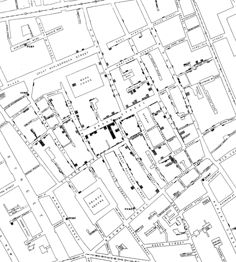
Snow (1855):

“… Each company supplies both rich and poor, both large houses and small; there is no difference in the condition or occupation of the persons receiving the water of the different companies… As there is no difference whatever either in the houses or the people receiving the supply of the two Water Companies, or in any of the physical conditions with which they are surrounded, it is obvious that no experiment could have been devised which would more thoroughly test the effect of water supply on the progress of Cholera than this, which circumstances placed ready made before the observer…”

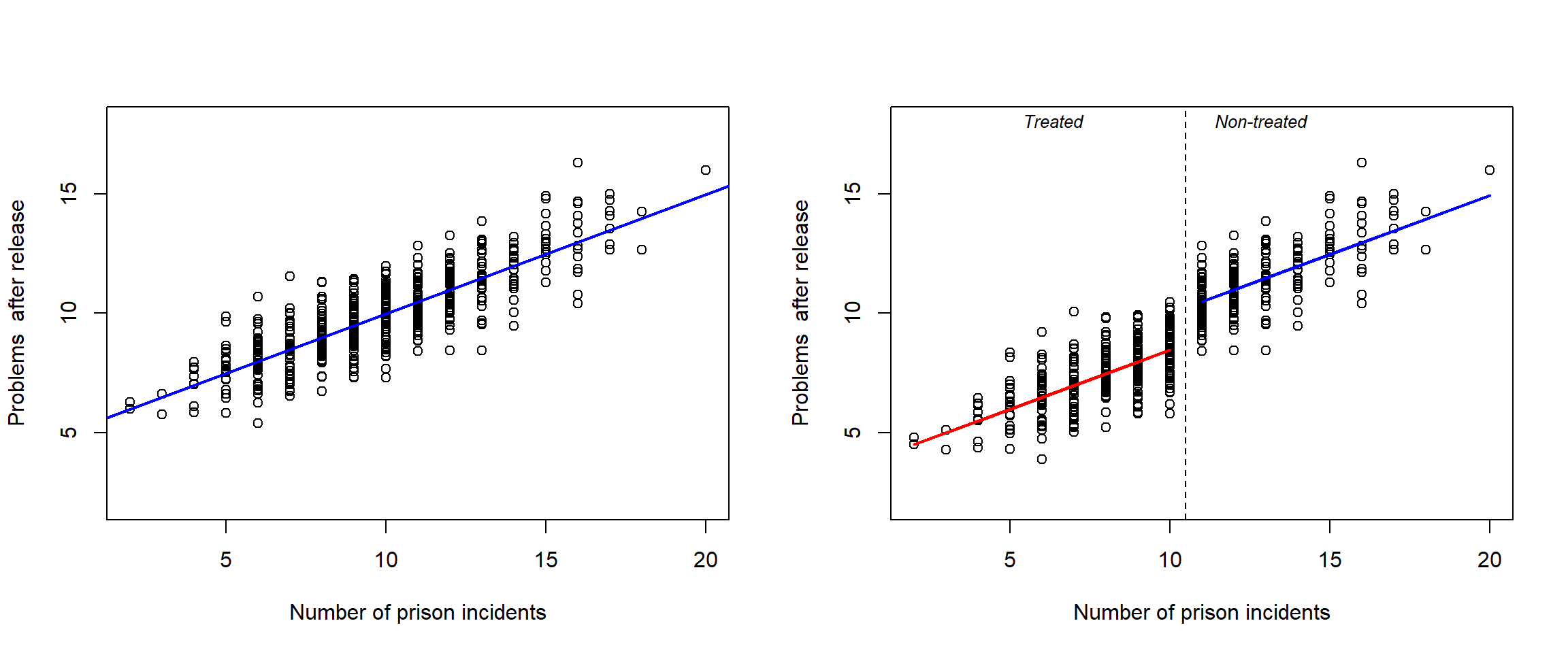
Regression discontinuity design, in theory a design with ignorable assignment mechanisms (under the strong assumption that its relationship to the outcome is modelled correctly, below assuming a linear relationship.)

Longitudinal studies

• Cohort studies: A group of people (cohort) who share characteristics, e.g., birth year, road-traffic noise exposure, work place, etc. are followed over time, and incidence of outcome (e.g., heart attack) is registered during the study period.
  • In terms of internal validity: Commonly consider the best observational-study design for causal inference
  • May be costly both in terms of sample size (if rare outcomes) and time (if outcomes take time to develop).
• Case-control studies: Select a group of people with the disease (outcome) and a comparison group without, and assess and compare their exsposures to the potential causal factor back in time.
  • Cost-efficient for rare outcomes
  • Recall bias may be a threat

Cross-sectional studies

Measuring both independent variables (exposure, covariates) and dependent variable (outcome) at the same time in a population (or sample) at one point in time.

• Easy to conduct in short time
• Reversed causation a major threat (apart from confounding and selection bias)
• Mono-method bias a major threat in studies using a single measuring instrument (e.g., a single questionnaire, as all too often seen in social science research).

13.3 Control for, adjust for, conditioning on, …

With the purpose to achieve other things equal (ceteris paribus).

• Repeated measures of single unit
• Matching on background variables
• Random assignment to treatment groups
• Restriction or stratification on background variables
• Statistical control

Matching

Goal: Unit homogeneity = exchangeable units

• As part of design (before data collection)
• May be used together with random assignment
• After data has been collected: Data pruning
• Strength: Model independent

Restriction or stratification on background variables

Restriction may increase internal validity, at the expense of external validity

• As part of design (before data collection), restrict data collection to a specific group, or make focus on several subgroups (e.g., age groups) and make sure to have enough data in each group for separate analysis.
• After data has been collected: Analysis restricted to a specific subgroup, or separate analysis of data from subgroups (of enough observations within subgroup)
• Strength: Model independent

Statistical control

Add covariates in a regression model.

Weakness: Model dependent, i.e., based on assumptions of, for example, linear relationships between variables (as assumed in multiple linear regression). If critical relationships are non-linear, for example, between confounders and the exposure, then confounding may still bias the causal effect estimate although the confounding variables have been included in the linear regression model (so called “residual confounding”)

13.4 Bias in observational studies

Confounding bias

Confounding, also known as “omitted variable bias” is maybe the most obvious alternative explanation to causal explanations. A third variable, not controlled for, may have influenced both exposure and outcome, leading to biased estimates of the causal effect.

A simple example: Hearing impairment is more common among construction workers than office workers. A potential causal factor is occupational noise exposure; after all, construction sites tend to be noisier than offices. But socioeconomic status is a potential confounder. Individuals from low socioeconomic background may be more likely to become construction workers than individuals from high socioeconomic background, and we know that socioeconomic status is related to most health outcomes, probably also risk for hearing impairment. Here is a simple DAG:

confound <- dagitty( "dag {
   Occupational_Noise -> Hearing_Impairment
   Occupational_Noise <- Socioeconomic_Status-> Hearing_Impairment
}")

coordinates(confound) <- list(
  x = c(Occupational_Noise = 1, Socioeconomic_Status = 2, Hearing_Impairment = 3),
  y = c(Occupational_Noise = 2, Socioeconomic_Status = 1, Hearing_Impairment = 2))

plot(confound)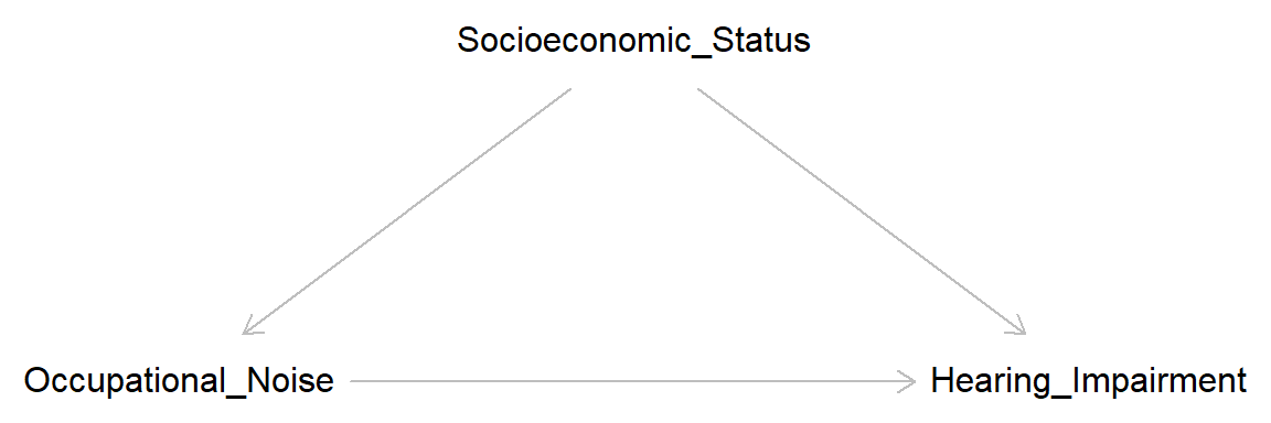

Note that according to this DAG, occupational noise do indeed cause hearing impairment, but the size of the causal effect may be biased unless variation in socioeconomic status is taken into account.

Negative confounding

A confounder may hide or mask a casual relationship between two variables. Consider this DAG:

confound2 <- dagitty( "dag {
   X -> Y
   X <- Z -> Y
}")

coordinates(confound2) <- list(
  x = c(X = 1, Z = 2, Y = 3),
  y = c(X = 2, Z = 1, Y = 2))

plot(confound2)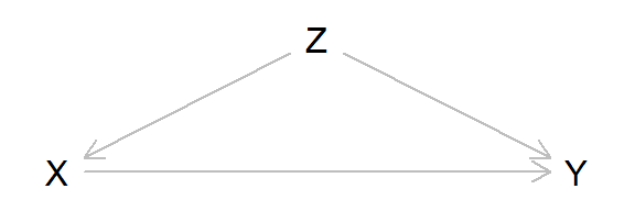

Here a simple simulation, assuming that the average causal effect of X on Y is 0.5, that is, increasing X with one unit would on average increase Y with 0.5 units.

set.seed(123)
n <- 1e5

# Define causal effects
b_zx <- -1 # Causal effect of z on x
b_zy <-  1   # Causal effect of z on y
b_xy <- 0.5  # Causal effect of x on y

# Define variables (structural equations)
z <- rnorm(n)
x <- rnorm(n) + b_zx*z
y <- rnorm(n) + b_zy*z + b_xy*x

# Try this if you prefer random effects:
# x <- rnorm(n) + rnorm(n, mean = b_zx, sd = 0.2) * z
# y <- rnorm(n) + rnorm(n, mean = b_zy, sd = 0.2) * z + 
#       rnorm(n, mean = b_xy, sd = 0.2) *x

# Estimate total average causal effect of x on y
lm_crude    <- lm(y ~ x)  # Crude model
lm_adjusted <- lm(y ~ x + z)  # Model adjusted for z

# Print results
lm_crude

Call:
lm(formula = y ~ x)

Coefficients:
(Intercept)            x  
   0.002486     0.003130  

lm_adjusted

Call:
lm(formula = y ~ x + z)

Coefficients:
(Intercept)            x            z  
 -0.0005948    0.5000543    0.9979861  

… and it may also reverse the causal effect estimate (type S error):

set.seed(123)
n <- 1e5

# Define causal effects
b_zx <- -1 # Causal effect of z on x
b_zy <-  1.5   # Causal effect of z on y
b_xy <- 0.5  # Causal effect of x on y

# Define variables (structural equations)
z <- rnorm(n)
x <- rnorm(n) + b_zx*z
y <- rnorm(n) + b_zy*z + b_xy*x

# Estimate total average causal effect of x on y
lm_crude    <- lm(y ~ x)  # Crude model
lm_adjusted <- lm(y ~ x + z)  # Model adjusted for z

# Print results
lm_crude

Call:
lm(formula = y ~ x)

Coefficients:
(Intercept)            x  
    0.00403     -0.24583  

lm_adjusted

Call:
lm(formula = y ~ x + z)

Coefficients:
(Intercept)            x            z  
 -0.0005948    0.5000543    1.4979861  

Residual confounding

Residual confounding is bias that remains despite our attempt to adjust for a confounder. This could happen for several reasons, for example:

• Our measure may not cover important aspects of the construct. Socioeconomic status measured by income may not capture aspects related to education, parents income, or socioeconomic status at the neighborhood level (living in an wealthy area of town may have beneficial consequences on health independent of socioeconomic status at the individual level).
• Adding a confounder to a regression model may not be enough because the relationship assumed by the model (e.g., linear) may not be a good approximation of the true relationship. Methods like matching or restriction are less vulnerable in this regard as they are model independent (make no assumptions about functional relationships between covariate and outcome).
• Restriction not tight enough, for instance, if analysis are restricted to adults younger than 40 years old, this may not be enough to adjust for age as there may still be an effect of age on exposure and outcome in this age span.

Why not control for all my covariats, how can I loose?

A key insight from learning about Directed Acyclic Graphs (DAGs) is that controlling for covariates can sometimes introduce bias. This can occur in two main ways: by controlling for a mediating variable, leading to overadjustment bias, or by controlling for a collider variable, resulting in collider bias. It’s also important to note that controlling for a descendant of such variables can similarly introduce bias, though typically to a lesser degree.

Overadjustment bias

“Overadjustment bias” or “overcontrol bias” refer to bias that is introduced by controlling for a mediating variable. In the example discussed above, controlling for hearing protection at work may lead to bias. Possibly overestimating the total average causal effect by eliminating a mediator that might reduce the adverse effect.

overadj <- dagitty( "dag {
   Occupational_Noise -> Hearing_Impairment <- Hearing_Protection
   Occupational_Noise -> Hearing_Protection
   Occupational_Noise <- Socioeconomic_Status-> Hearing_Impairment
}")

coordinates(overadj) <- list(
  x = c(Occupational_Noise = 1, Socioeconomic_Status = 2, Hearing_Protection = 2, 
        Hearing_Impairment = 3),
  y = c(Occupational_Noise = 2, Socioeconomic_Status = 1, Hearing_Protection = 1.5,
        Hearing_Impairment = 2))

plot(overadj)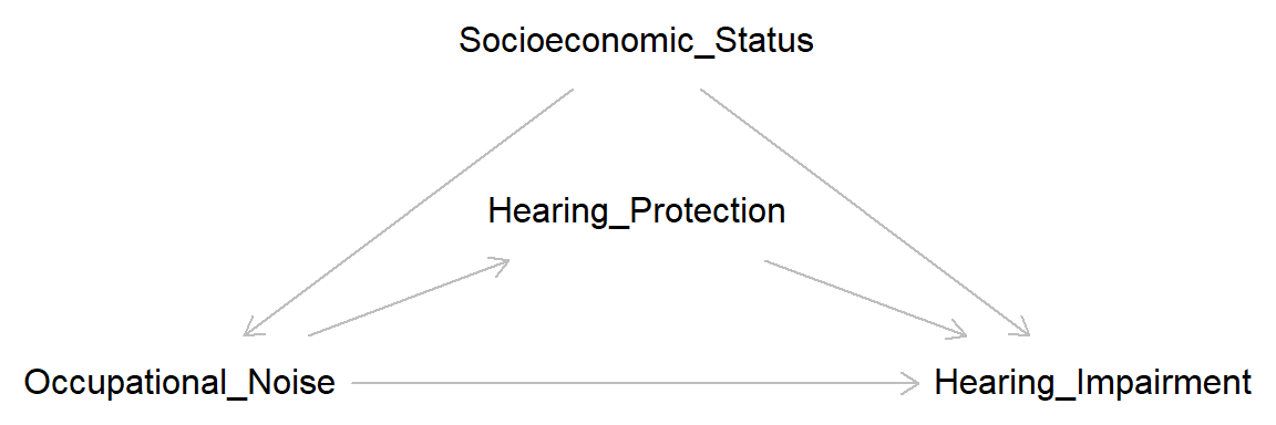

Collider bias

Conditioning on a variable that is a collider may introduce bias. In this DAG, Stress (physiological reactivity to stressors) is a collider on the path

\(Occupational \ Noise \rightarrow Stress \leftarrow Genetic \rightarrow Hearing \ Impariment\),

where Genetic may be some unmeasured biological vulnerability linked to both physiological stress reactions and hearing impairment. Adjusting for Stress may introduce collider bias by opening up a backdoor path between exposure and outcome.

collide <- dagitty( "dag {
   Occupational_Noise -> Hearing_Impairment <- Hearing_Protection
   Occupational_Noise -> Hearing_Protection
   Occupational_Noise <- Socioeconomic_Status-> Hearing_Impairment
   Occupational_Noise -> Stress <- Genetic -> Hearing_Impairment
}")

coordinates(collide) <- list(
  x = c(Occupational_Noise = 1, Socioeconomic_Status = 2, Hearing_Protection = 2, 
        Hearing_Impairment = 3, Stress = 2, Genetic = 2.5),
  y = c(Occupational_Noise = 2, Socioeconomic_Status = 1, Hearing_Protection = 1.5,
        Hearing_Impairment = 2, Stress = 2.75, Genetic = 2.5))

plot(collide)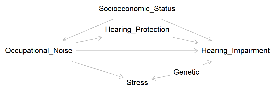

Here a simple example of collider bias:

\(Intelligence \rightarrow Income \leftarrow Social \ skills\)

Assume that intelligence is independent of social skills in the general population, and that both have a positive influence on income. Assume we found a negative association between IQ scores and scores on a social skill test in a sample of chief executive officers (CEOs) of large companies. A causal interpretation of this could be that: “Maybe people with high IQ spend a lot of time reading books, and therefore do not develop their social skills.” An alternative explanation would be that the observed association was spurious, an example of collider bias. Here a simulation:

set.seed(431)
n <- 3e3
iq <- rnorm(n) # IQ scores, standardized to mean = 0, sd = 1
ss <- rnorm(n)  # Social skill scale, standardized to mean = 0, sd = 1
income <- rnorm(n) + rnorm(n, 0.4, 0.2) * iq  +rnorm(n, 0.4, 0.2) * ss

# Plot full popualtion
plot(iq, ss, xlab = "Intelligence (z-score)", ylab = "Social skills (z-score)")
abline(lm(ss ~iq))

# Add line for sample restricted to high income people
points(iq[income > 2], ss[income > 2], pch = 21, bg = "blue")
abline(lm(ss[income > 2] ~iq[income > 2]), lty = 2, col = "blue")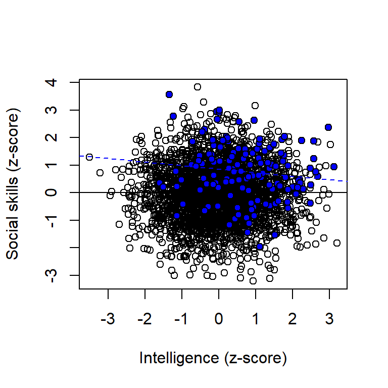

Open symbols and black regression line refer to the full population; blue points and blue regression line refer to a sample restricted to high income people.

Bias summary

Assume that we observed that X and Y were associated in our sample. “X cause Y” (H1) is certainly not the only possibility, here is my list of potential explanations (I am sure you can find more examples):

• H0: Sampling error: X and Y are not causally related, or otherwise associated in the population.
  • Possible DAG: \(X \rightarrow Z, \ \ Y \leftarrow W\)
• H1: Causation: X causes Y.
  • Possible DAG: \(X \rightarrow Z \rightarrow Y\)
• H2: Reversed causation: Y causes X.
  • Possible DAG: \(X \leftarrow Z \leftarrow Y\)
• H3: Confounding: Z causes both X and Y
  • Possible DAG: \(X \leftarrow Z \rightarrow Y\)
• H4: Collider bias: X and Y both causes Z and we have conditioned on Z (e.g., if Z is income and our sampel only included individuals with high income).
  • Possible DAG: \(X \rightarrow \boxed{Z} \leftarrow Y\)

Assume that we observed that X and Y were not associated in our sample. “X does not cause Y” (H0) is certainly not the only possibility, here is my list of potential explanations (I am sure you can find more examples):

• H0: Independence: X and Y are not causally related, or otherwise associated in the population.
  • Possible DAG: \(X \rightarrow Z, \ \ Y \leftarrow W\)
• H1: Causation masked by sampling error: X causes Y
  • Possible DAG: \(X \rightarrow Z \rightarrow Y\) (Note that DAGs assume error free variables.)
• H2: Reversed causation masked by sampling error: Y causes X
  • Possible DAG: \(X \leftarrow Z \leftarrow Y\) (Note that DAGs assume error free variables.)
• H3: Causation masked by conditioning on a mediator: X causes Y
  • Possible DAG: \(X \rightarrow \boxed{Z} \rightarrow Y\)
• H4: Reversed causation masked by conditioning on a mediator: Y causes X
  • Possible DAG: \(X \leftarrow \boxed{Z} \leftarrow Y\)
• H5: Negative confounding: X causes Y, masked by negative confounding of Z
  • Possible DAG: \(X \leftarrow Z \rightarrow Y, \ \ X \rightarrow Y\) (Note that DAGs assume that perfect cancellation is not the case. Still, the observed association may be very weak suggesting a negligable association despite a sizebale causal relationship between X and Y).
• H6: Negative confounding and reversed causation: Y causes X, masked by negative confounding of Z (Note comment on H5)
  • Possible DAG: \(X \leftarrow Z \rightarrow Y, \ \ X \leftarrow Y\)
• H7: Collider bias X causes Y, masked by collider bias due to conditioning on common effect Z.
  • Possible DAG: \(X \rightarrow \boxed{Z} \leftarrow Y, \ \ X \rightarrow Y\)
• H8: Collider bias and reversed causation Y causes X, masked by collider bias due to conditioning on common effect Z.
  • Possible DAG: \(X \rightarrow \boxed{Z} \leftarrow Y, \ \ X \leftarrow Y\)

13.5 Why experiments are superior to observational studies for causal inference

The simple DAG answer: Experiments disconnect the exposure variable (X) from other variables in the causal diagram, that is, the manipulation changes X from being an endogenous variable to an exogenous variable. Assuming of course that assignment mechanism, non-compliance and missing data are “ignorable”.

Short-cut DAG:

The full DAG may be hard to conceptualize, for example if the research field is not well-developed with little theory to guide the construction of the full DAG. A short-cut is then to conceptualize all casual paths leading in to X and then try to close these by conditioning on relevant variables, mimicking an experiment where X is manipulated.

Closing all paths going in to X is, in theory, analogous to manipulating X.

shortcut <- dagitty( "dag {
   W -> Z1 -> X
   Y <- V <- Z2 -> X <- W
   X -> M -> Y
   Y <- Z3 -> X
   Z2 <- Z4 -> X
   Z4 -> M
   
}")

coordinates(shortcut) <- list(
  x = c(W = 1, Z1 = 2, X = 3, V = 5, Z2 = 4, M = 4, Y = 5, Z3 = 4, Z4 = 2.5),
  y = c(W = 2, Z1 = 1, X = 1, V = 2, Z2 = 2, M = 1, Y = 1, Z3 = 1.5, Z4 = 1.5))

plot(shortcut)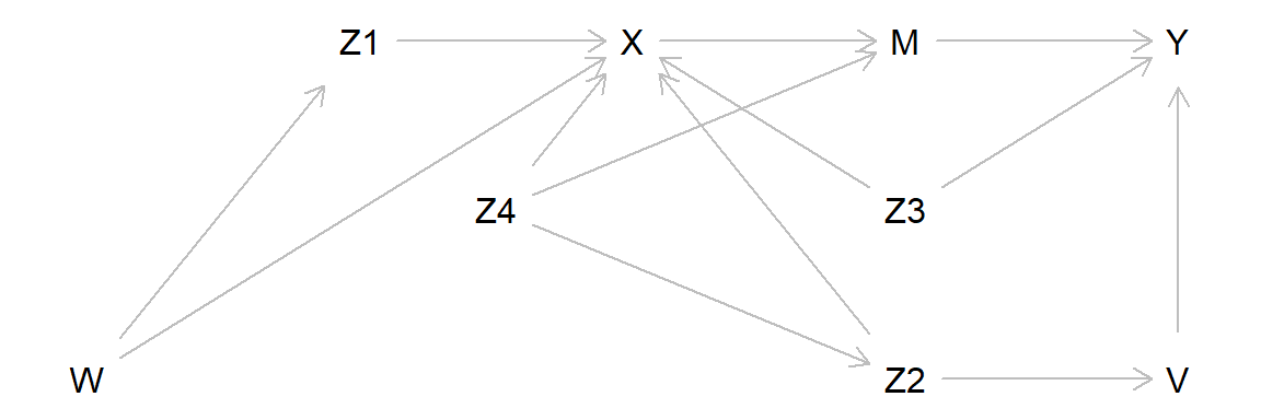

These are two helpful suggestions:

• Adjust for all pre-treatment variables. Doing so theoretically blocks all causal paths to the exposure variable, effectively eliminating confounding.

• Avoid adjusting for any post-treatment variables. As doing so can introduce overadjustment bias or collider bias.

Practice

The practice problems are labeled Easy (E), Medium (M), and Hard (H), (as in McElreath (2020)).

Easy

13E1.
Suppose that in the population of college applicants, being good at baseball is independent of having a good math score on a certain standardized test (with respect to some measure of ‘good’). A certain college has a simple admission procedure: admit an applicant if and only if the applicant is good at baseball or has a good math score or both. Give an intuitive explanation of why it makes sense that among students that this college admits, having a good math score is negatively associated with being good at baseball, i.e., conditioning on having a good math score decreases the chance of being good at baseball.

Old exam question (stolen from Blitzstein & Hwang, 2019, an excellent introduction to probability)

13E2. Adjustment of a mediator may lead to overadjustment bias or collider bias or both when estimating the total average causal effect of exposure on outcome. Explain.

13E3. Many observational studies on violent video gaming and aggression only include boys. Why may this be a good idea?

Medium

13M1. Draw a simple DAG illustrating confounding, and discuss how the sign of the relationships may lead to negative confounding.

13M2. Residual confounding is bias that remains despite our attempt to control for a confounder. Explain why residual confounding may be more of a problem if the covariate is controlled for by statistical control (adding it to a regression model) then by matching on the covariate.

13M3. When estimating causal effects in experiments or observational studies, including variables in a regression model is a way of adjusting for covariates. Two simple rules when estimating total causal effects:

Rule 1. Adjust for all measured pre-treatment covariates.
Rule 2. Don’t adjust for any post-treatment covariates.

1. Explain why Rule 1 is a good idea.
2. Explain why Rule 2 is a good idea.

Hard

13H1. Assume that X is a dichotomous variable that causes Y, and that Z causes both X and Y. Furthermore, assume that \(Z \rightarrow Y\) is non-linear (e.g., quadratic). Simulate data and estimate the total average causal effect of X on Y in two ways:

1. Statistical control: Add Z as covariate to the linear model: \(Y = b_0 + b_1X + b_2Z\).
2. Matching: Only include pairs of X = 0 and X = 1 with similar values on Z (matching as data pruning).

Discuss the two methods ability to recover the true casual effect for your simulated scenario.

13H2. Matching is an adjustment strategy that can be applied both at the design stage of a study and after data collection. When implemented after data collection, it is sometimes referred to as “data pruning.” Explain the rationale behind this terminology and discuss how matching differs when applied at the design stage versus after data collection.

13H3. Two rules were mentioned above (13M3):

Rule 1: Adjust for all measured pre-treatment covariates. Rule 2: Avoid adjusting for any post-treatment covariates.

These are excellent general guidelines. However, like most rules, they come with exceptions!

1. Draw a Directed Acyclic Graph (DAG) that represents a scenario where it would be beneficial to violate Rule 1.

2. Draw a Directed Acyclic Graph (DAG) that represents a scenario where it would be beneficial to violate Rule 2.

13H4. Researchers wanted to compare kids from a low and a high socioeconomic area on their response to a new pedagogic method for teaching math. They first administered a short math test to all kids in each area and noted the the average score among the kids from the high socioeconomic area was much higher than the average score among the kids from the low socioeconomic area. To achieve balanced groups, they took a random sample of 50 kids from the low socioeconomic area and then matched each kid with a kid from the high socioeconomic area with a similar score on the math test. Both groups were then subjected to the new pedagogic method, after which they were tested again on a similar test. The 50 low socioeconomic kids had about the same average result as before, whereas the 50 high socioeconomic kids had a higher average score after than before. The conclusion was that the method seems to work, but only for kids with a high socioeconomic background.

Give an alternative explanation.

(Session Info)

sessionInfo()

R version 4.4.2 (2024-10-31 ucrt)
Platform: x86_64-w64-mingw32/x64
Running under: Windows 11 x64 (build 26100)

Matrix products: default


locale:
[1] LC_COLLATE=Swedish_Sweden.utf8  LC_CTYPE=Swedish_Sweden.utf8   
[3] LC_MONETARY=Swedish_Sweden.utf8 LC_NUMERIC=C                   
[5] LC_TIME=Swedish_Sweden.utf8    

time zone: Europe/Stockholm
tzcode source: internal

attached base packages:
[1] stats     graphics  grDevices utils     datasets  methods   base     

other attached packages:
[1] dagitty_0.3-4

loaded via a namespace (and not attached):
 [1] digest_0.6.37     fastmap_1.2.0     xfun_0.52         knitr_1.50       
 [5] htmltools_0.5.8.1 rmarkdown_2.29    cli_3.6.5         compiler_4.4.2   
 [9] boot_1.3-31       rstudioapi_0.17.1 tools_4.4.2       curl_6.4.0       
[13] evaluate_1.0.3    Rcpp_1.0.14       yaml_2.3.10       rlang_1.1.6      
[17] jsonlite_2.0.0    V8_6.0.4          htmlwidgets_1.6.4 MASS_7.3-61      

Blitzstein, J. K., & Hwang, J. (2019). Introduction to probability. Chapman; Hall/CRC.

Elwert, F., & Winship, C. (2014). Endogenous selection bias: The problem of conditioning on a collider variable. Annual Review of Sociology, 40, 31–53.

McElreath, R. (2020). Statistical rethinking: A bayesian course with examples in r and stan. Chapman; Hall/CRC.

Rohrer, J. M. (2018). Thinking clearly about correlations and causation: Graphical causal models for observational data. Advances in Methods and Practices in Psychological Science, 1(1), 27–42.

Snow, J. (1855). On the mode of communication of cholera. John Churchill.